keras 线性回归预测

最新推荐文章于 2025-05-14 10:35:31 发布

原创最新推荐文章于 2025-05-14 10:35:31 发布 · 859 阅读

3 ·

CC 4.0 BY-SA版权

文章标签：

#线性回归

python 同时被 3 个专栏收录

62 篇文章

订阅专栏

深度学习

57 篇文章

订阅专栏

tensorflow

26 篇文章

订阅专栏

本文通过使用Keras实现线性回归模型，演示了如何从数据准备到模型训练及预测的全过程。文中详细介绍了利用Python及其相关库进行数据生成、模型搭建、训练以及最终结果的可视化展示。

摘要生成于 C知道，由 DeepSeek-R1 满血版支持，前往体验 >

#!/usr/bin/env python
# -*- coding:UTF-8 -*-
import numpy as np
np.random.seed(1337)  # for reproducibility
from keras.models import Sequential
from keras.layers import Dense
import matplotlib.pyplot as plt 
# 可视化模块

X = np.linspace(-1, 1, 200)
np.random.shuffle(X)    # randomize the data
Y = 0.9 * X + 2 + np.random.normal(0, 0.05, (200, ))
# plot data
#plt.scatter(X, Y)
#plt.show()
 
X_train, Y_train = X[:160], Y[:160]     # train 前 160 data points
X_test, Y_test = X[160:], Y[160:]       # test 后 40 data points
#plt.plot(X_train, Y_train,'.')
#plt.show()

model = Sequential()
l1 = Dense(output_dim = 1,input_dim = 1)
model.add(l1)

model.compile(loss = 'mse',optimizer = 'sgd')
model.fit(X_train,Y_train,epochs= 3000)

print(l1.get_weights())
Xe = np.linspace(1, 2, 20)
Ye = model.predict(Xe)

plt.plot(X_train, Y_train,'.',Xe,Ye,'.')
plt.show()

运行结果

Epoch 3000/3000
160/160 [==============================] - 0s 30us/step - loss: 0.0026
[array([[0.8913625]], dtype=float32), array([2.0040555], dtype=float32)]
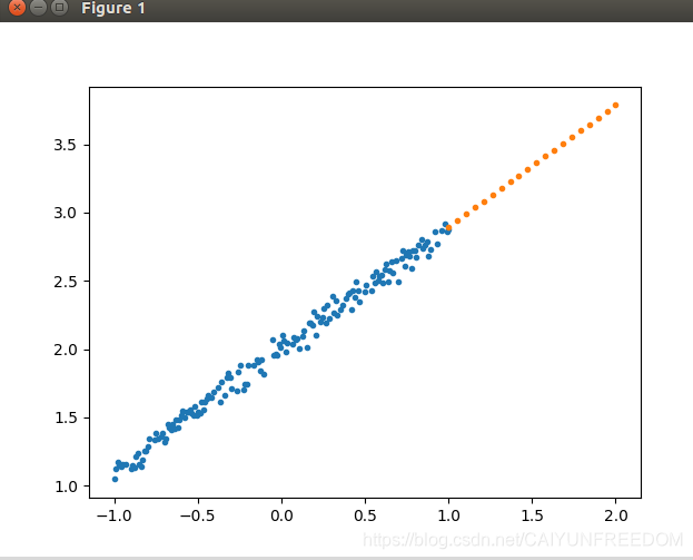
训练得到的权重和偏置和理论值0.9 2 很接近了。

下图中橙色点是预测部分，蓝色点是训练数据。