


 该博客围绕JPEG编解码实验展开,介绍了实验目的,即掌握JPEG编解码原理与数据压缩算法实现。阐述了JPEG编码器、解码器原理及文件解析方法,还说明了实验内容,包括调试理解解码器程序、理解程序设置、输出量化表和huffman表以及DC、AC图像及其概率分布。
目录
一、实验目的
掌握JPEG编解码系统的基本原理。初步掌握复杂的数据压缩算法实现,并能根据理论分析需要实现所对应数据的输出。
二、实验原理
(本来打算和电视原理讲的JPEG结合一下,最后总结的太乱了,大家还是看图吧)
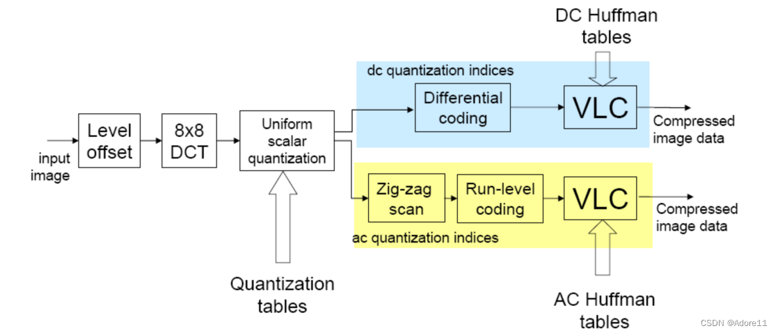
1、JPEG编码器: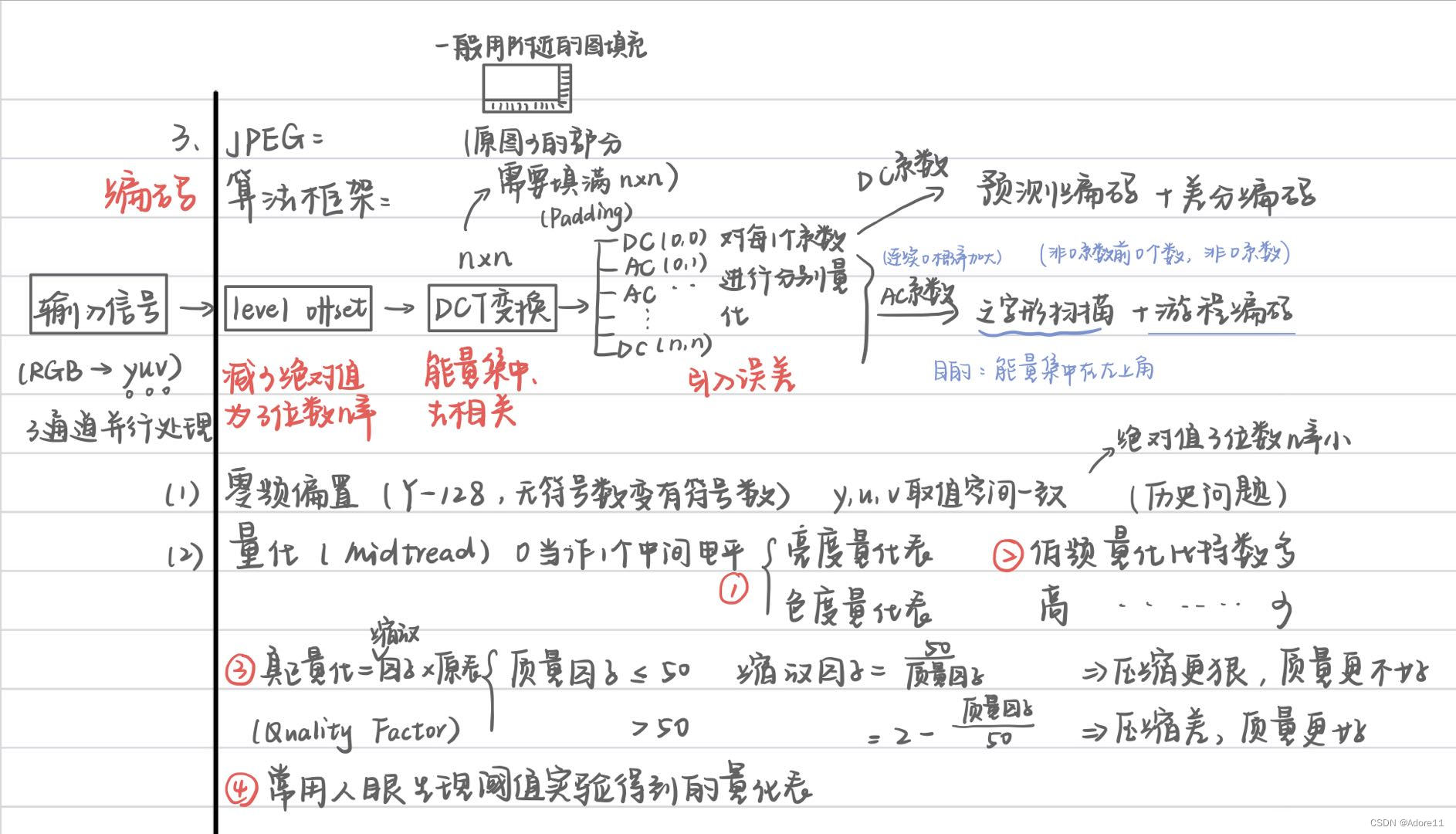
(1)零频偏置:(由单极性信号转变为双极性信号)
——为了减少绝对值为三位数的几率,将0电平移动到中央,降低平均亮度,降低DCT变化变化后的直流系数。
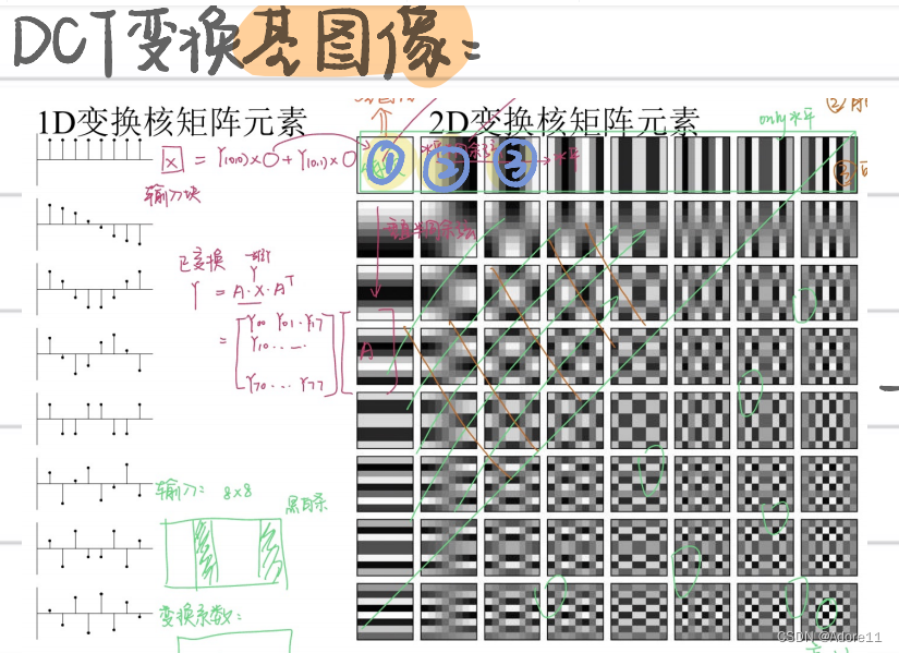
(2)DCT变换:(注意这里是无损变换)
去除数据图像的相关性,使图像能量集中,去除信号之间相关性。
——注意DCT的物理变化~(信号的合成和分解)
(3)量化:(引入误差)
⚪由于人眼对亮度信号比对色差信号更敏感,JPEG针对亮度和色度使用了两种不同量化表(色度量化表、亮度量化表)
⚪考虑到人眼对低频敏感,对高频不太敏感的视觉特性,低频部分采取较细量化,高频部分采取粗量化,减少视觉冗余。
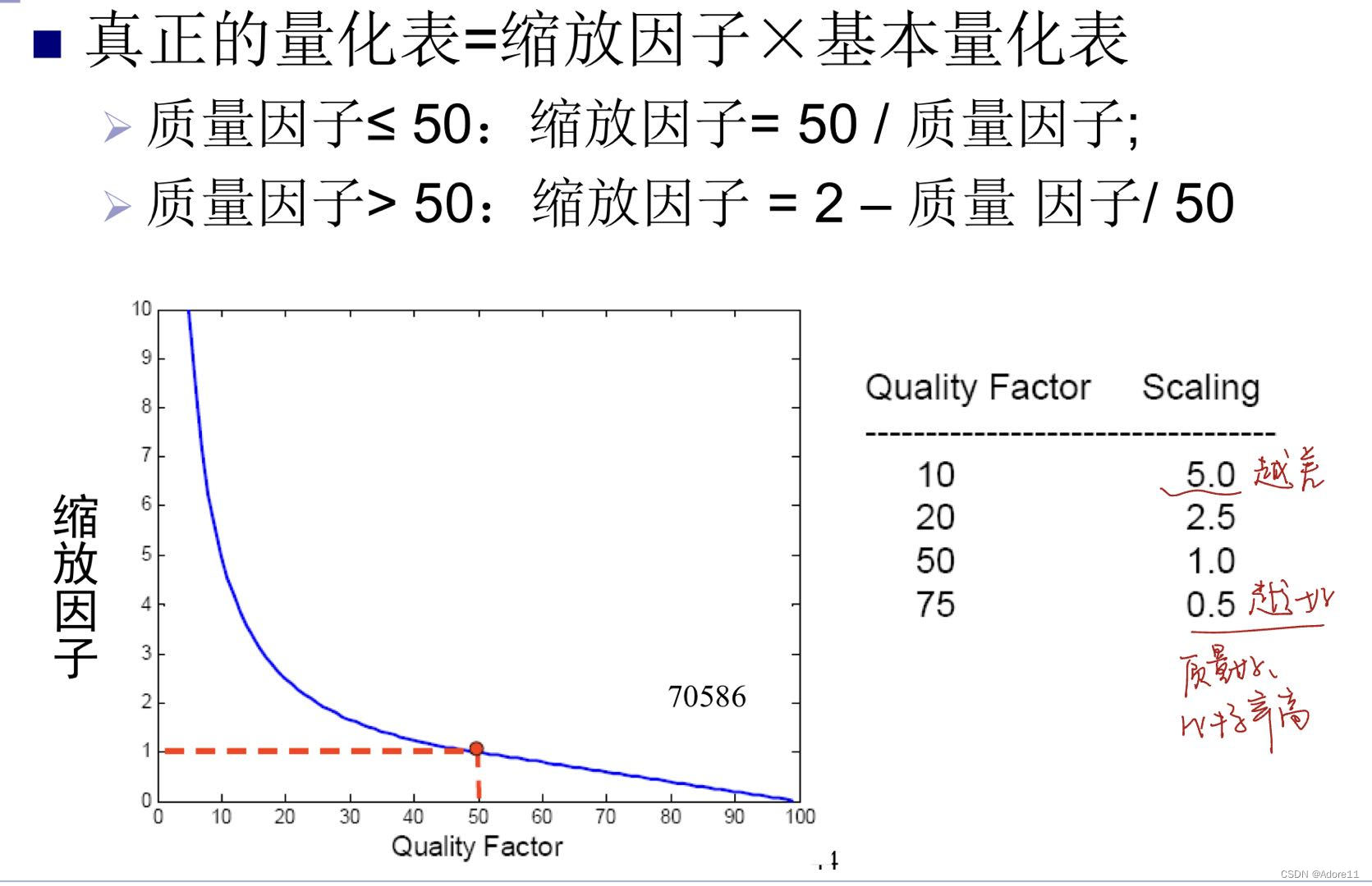
⚪同时JPEG还引入了缩放因子,真正的量化表=缩放因子*基本量化表,质量因子越小,量化程度越深,图像质量越不好。
(4)DC系数DPCM差分编码
考虑到DCT变换后(能量集中在左上角低频分量的特点):①DC系数大,②相邻的DC系数之间变化不大(存在冗余)的特征,对DC系数采用差分预测编码的方式
(5)AC系数(之字形扫描+游程编码)
同样考虑到DCT变换后,系数集中在左上角低频分量区,因此采用之字形按频率读出能够出现很多连零的机会。利用重复零可以进行游程编码进一步增加压缩效率。(游程编码非本次课程重点,理解原理即可)
注意:AC系数按照之字形存储,量化表中的系数也是按照之字形存储!!!!!
(6)Huffman编码
DC和AC系数分别进行Huffman编码,最终输出编码后的图像
2、JPEG解码器
可以理解为编码的逆过程。
解码熵编码——重构量化后系数——反DCT——丢弃填充的行列——反0偏置——下采样逆过程——转RGB图像
3、JPEG文件解析
用Visual Studio二进制编辑器格式打开一个jpeg文件:
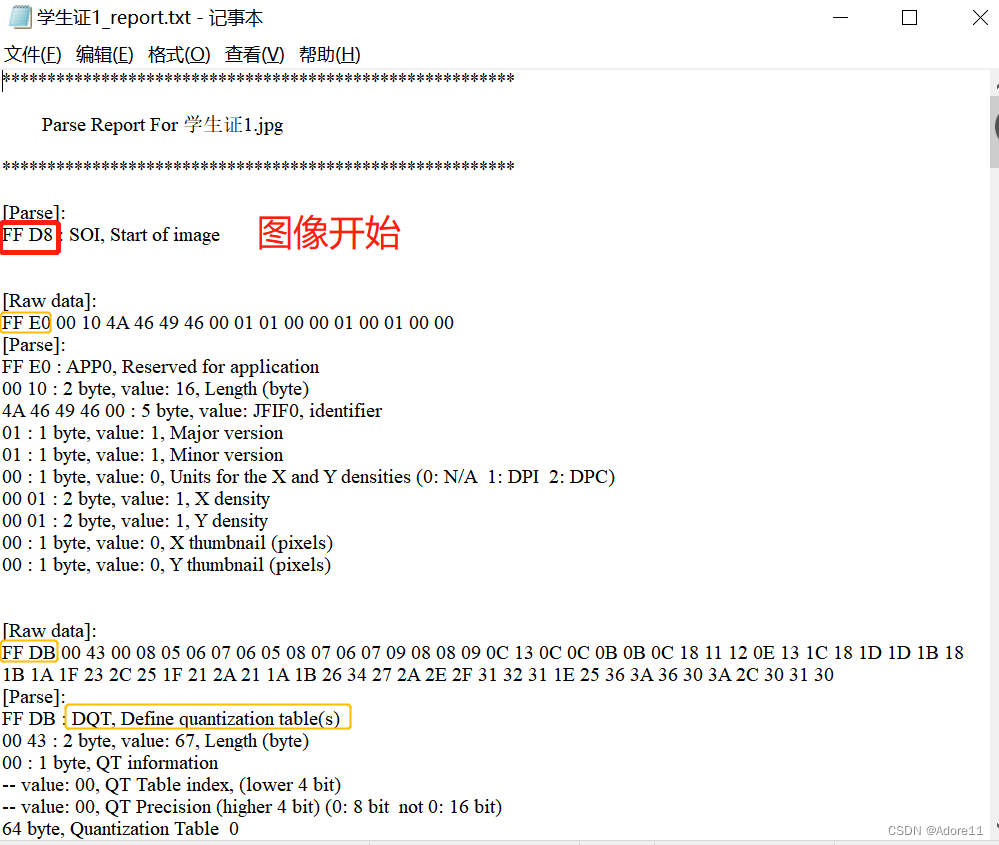
(1)SOI ,Start of Image图像开始:固定标识符0xFFD8 (每一个JPEG文件都必须以SOI开始)
![]()
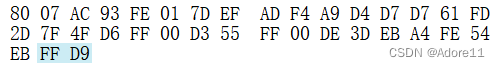
(2)EOI,End of Image图像结束:固定标识符0xFFD9
(3)APP0 应用程序保留标记0
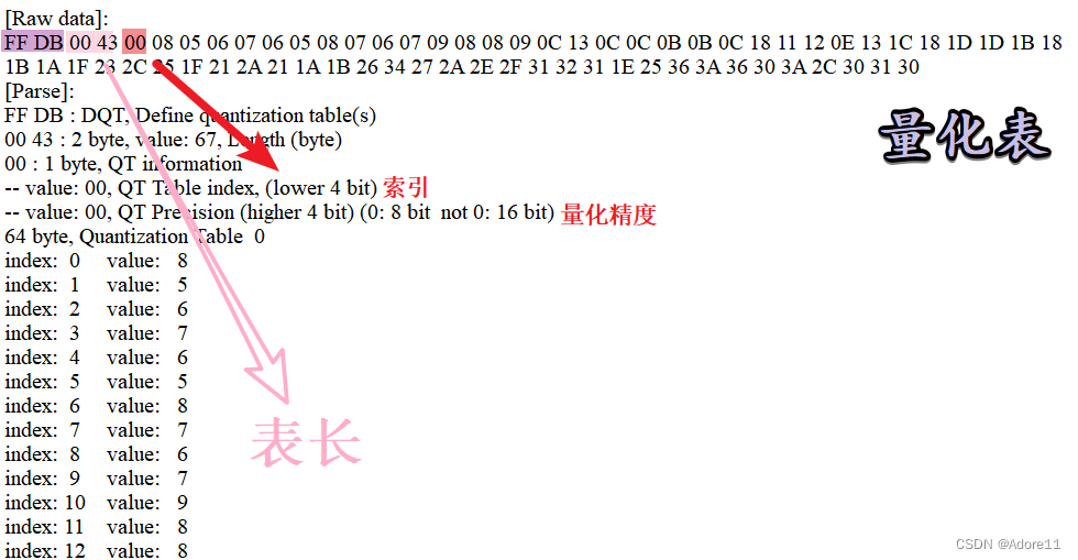
(4)DQT 定义量化表:固定标识符0xFFDB
可以重复出现,表示多个量化表,一般为两个量化表(AC&DC),如下图所示
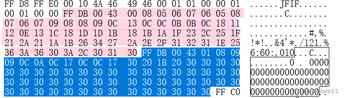
略展开说一说:JPEG中量化表也是按照之字形存储,0043表示表长,00(0表示精度,C表示index,这里是序号是0的量化表)剩下64bytes分别表示量化表的量化系数:
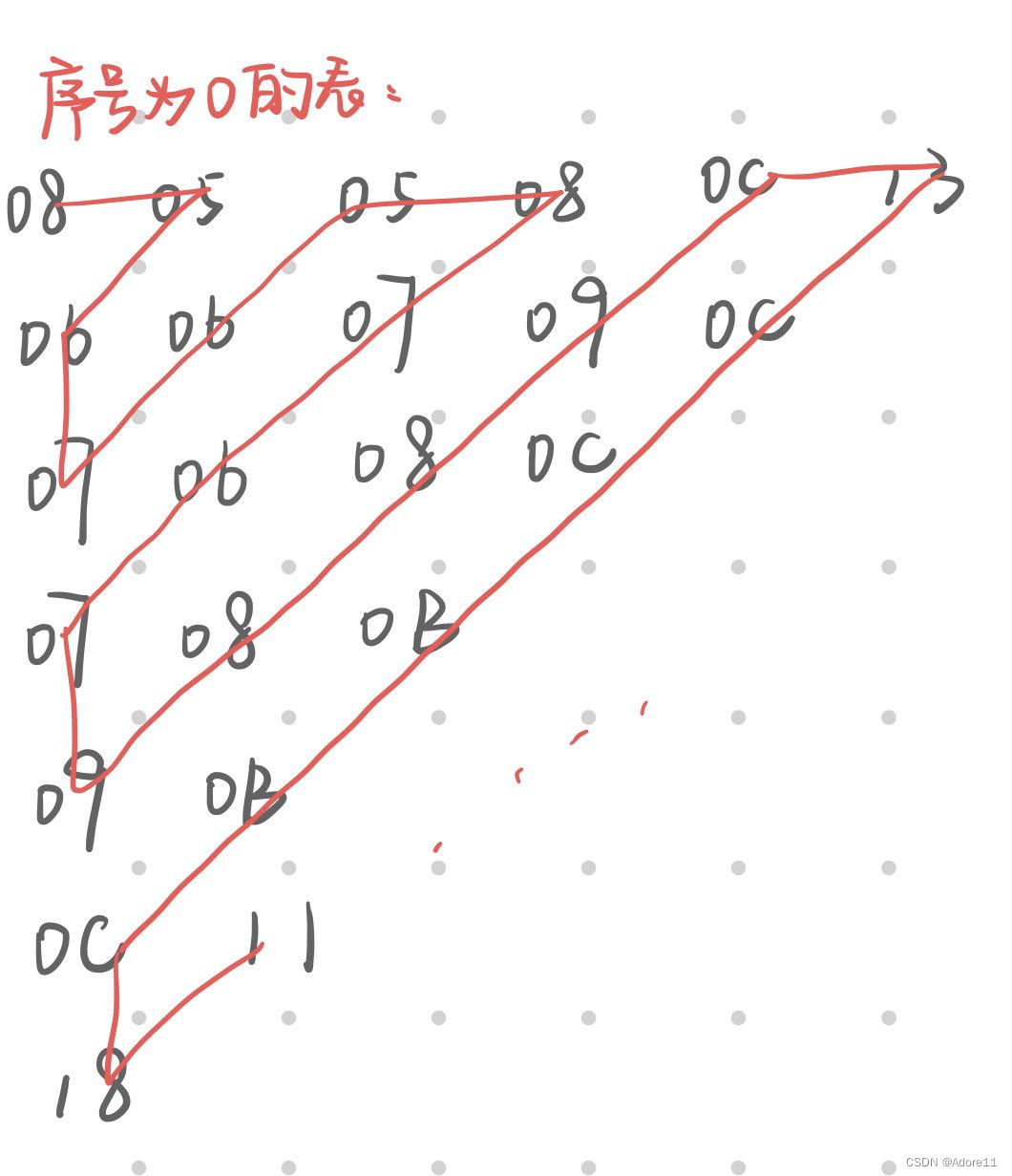
将序号为0的量化表反之字形输出:
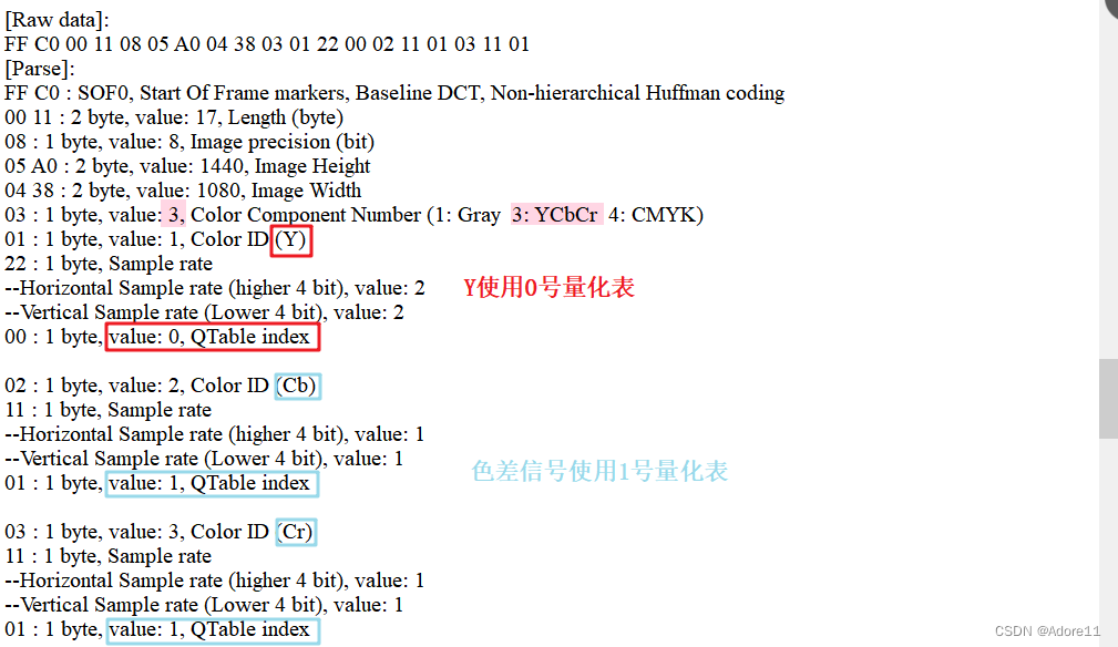
(5) SOF0一帧图像的开始,固定标识符0xFFC0
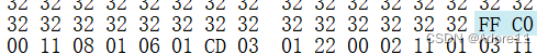
长度:0x0011,精度08(每个颜色分量每个像素1byte),图像高度0x0801,图像宽度(0x0601)
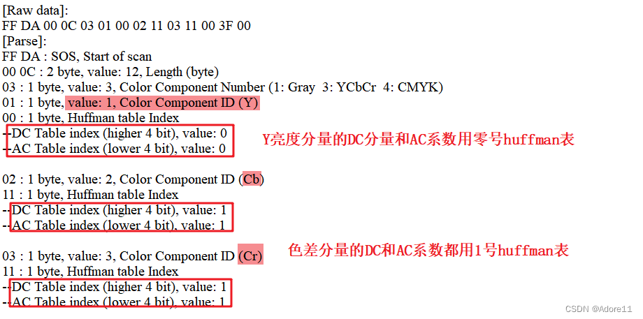
(6)DHT:哈夫曼表,固定标识符0xFFC4
通常会有4个DHT表,分别用于表示AC的亮度、色度;DC的亮度、色度
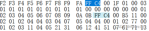
001F表长,01高四bit表示表示DC,低四bit为1号表,后续按照huffman标准化编码表示
三、实验内容
(1)调试和理解JPEG解码器程序
将输入的JPEG文件进行解码,将输出文件保存为可供YUVViewer观看的YUV文件。
1、将JPEG图放到JPEG_parser程序中,输出JPEG图的详细信息,对信息进行分析:
2、查看JPEG编解码cpp文件进行分析
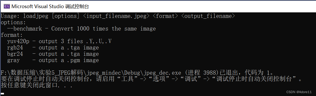
①查看命令行参数:(不设置命令行参数,运行程序)
options:需要输入三个命令行参数
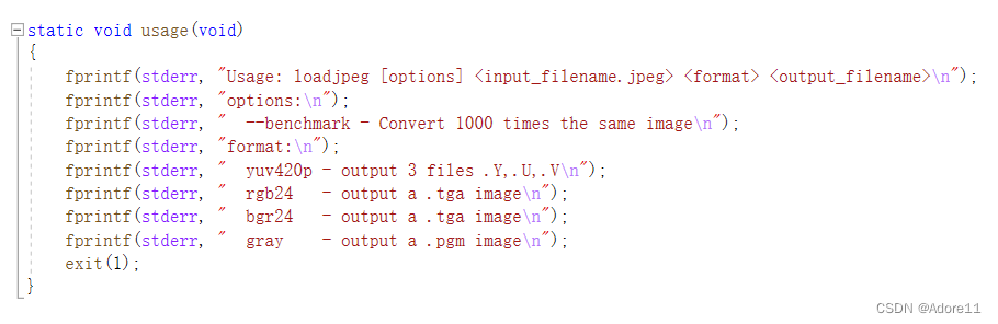
loadjpeg [options] <input_filename.jpeg> <format> <output_filename>
输入的jpg图像名称、jpeg图像格式、输出的文件名称(图像格式如下:yuv、rgb、bgr、gray)
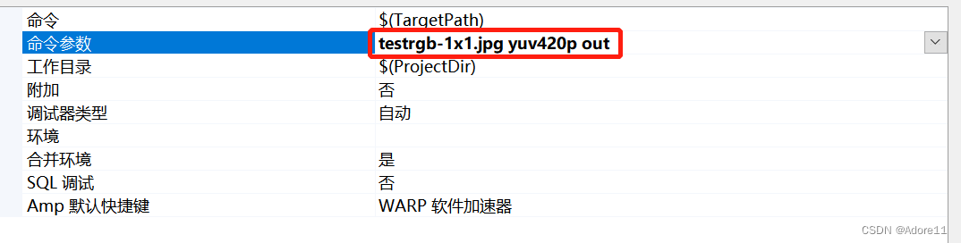
②设置命令行参数
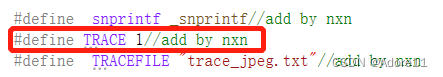
③观察程序中TRACE
最开始TRACE的定义写在头文件tinyjpeg.h中,初始化为1
后来在程序中很多地方都有trace的调用,随机选取一个分析
如果 trace=1,以写入的方式打开tracefile的文件目录,接着检查trace指针的状态;
trace方便我们的程序边运行边将运行结果写入文档,我们能通过文档判断程序是否正确解码。
(2)理解程序设置
1、结构体理解
在理解程序之前,我们先简单认识一下程序中最开始定义的三个结构体
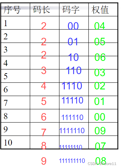
①huffman table:存储huffman码表
struct huffman_table/////定义huffman码表结构
{
  /* Fast look up table, using HUFFMAN_HASH_NBITS bits we can have directly the symbol,
   * if the symbol is <0, then we need to look into the tree table */
  short int lookup[HUFFMAN_HASH_SIZE];!!!!获取权值对应的码字
  /* code size: give the number of bits of a symbol is encoded */
  unsigned char code_size[HUFFMAN_HASH_SIZE];!!!!码长
  /* some place to store value that is not encoded in the lookup table
   * FIXME: Calculate if 256 value is enough to store all values
   */
  uint16_t slowtable[16-HUFFMAN_HASH_NBITS][256];//还存储一个大型huffman表?当当码长>9时,由该表处理
};
正常huffman码表解码时需要的码表结构如下图:
②component:存储解码信息,包括采样因子、量化表信息、以及AC和DC系数的指针等。
struct component
{
  unsigned int Hfactor;// 水平采样因子
  unsigned int Vfactor;// 垂直采样因子
  float *Q_table;	   // 8*8块的量化表
  struct huffman_table *AC_table;// AC交流系数的huffman码表
  struct huffman_table *DC_table;// DC直流系数的huffman码表
  short int previous_DC;	//获取前一个块解码后的DC系数(考虑到后面的DPCM编码,需要保存上一个块的像素值
  short int DCT[64];		//DCT系数
#if SANITY_CHECK
  unsigned int cid;
#endif
};
③jdec_private:定义JPEG数据流信息,声明图像数据、量化表、Huffman表、DCT解码后系数存储空间等。
struct jdec_private
{
  /* Public variables */
  uint8_t *components[COMPONENTS];//定义指针数组,指向三种分量用于存放解码后数据的数组的地址
  unsigned int width, height;//图像宽高
  unsigned int flags;

  /* Private variables */
  const unsigned char *stream_begin, *stream_end;//标记数据流的开始和结束
  unsigned int stream_length;//数据流长度

  const unsigned char *stream;	                //当前解码流指针
  unsigned int reservoir, nbits_in_reservoir;//数据流长度

  struct component component_infos[COMPONENTS];//存放三种分量的component信息
  float Q_tables[COMPONENTS][64];		        /* quantization tables */
  struct huffman_table HTDC[HUFFMAN_TABLES];	/* DC huffman tables   */
  struct huffman_table HTAC[HUFFMAN_TABLES];	/* AC huffman tables   */
  int default_huffman_table_initialized;
  int restart_interval;
  int restarts_to_go;				/* MCUs left in this restart interval */
  int last_rst_marker_seen;			/* Rst marker is incremented each time */

  /* Temp space used after the IDCT to store each components */
  uint8_t Y[64*4], Cr[64], Cb[64];//保存每个块经过IDCT解码后的像素

  jmp_buf jump_state;
  /* Internal Pointer use for colorspace conversion, do not modify it !!! */
  uint8_t *plane[COMPONENTS];//用于彩色空间转换
};
2、梳理代码逻辑
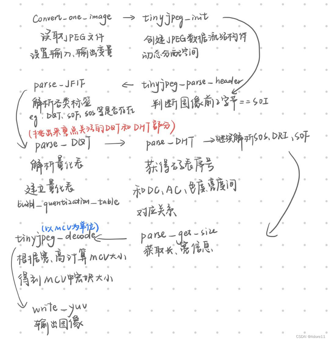
convert_one_image函数(读取判断输入文件格式,解码并按照输出格式输出)
int convert_one_image(const char *infilename, const char *outfilename, int output_format)
{//输入文件名称、输出文件名称、输出文件格式
  FILE *fp;
  unsigned int length_of_file;  // 文件大小
  unsigned int width, height;   // 图像宽、高
  unsigned char *buf;
  struct jdec_private *jdec; //JPEG数据数据流
  unsigned char *components[3];

  fp = fopen(infilename, "rb");//读取JPEG图像
  if (fp == NULL)
    exitmessage("Cannot open filename\n");
  length_of_file = filesize(fp);//输入文件的字节大小
  buf = (unsigned char *)malloc(length_of_file + 4);
  if (buf == NULL)
    exitmessage("Not enough memory for loading file\n");
  fread(buf, length_of_file, 1, fp);
  fclose(fp);

  /* Decompress it */
  jdec = tinyjpeg_init();   // 初始化
  if (jdec == NULL)
    exitmessage("Not enough memory to alloc the structure need for decompressing\n");

  if (tinyjpeg_parse_header(jdec, buf, length_of_file)<0)//读取头文件,检查图像格式
    exitmessage(tinyjpeg_get_errorstring(jdec));

  tinyjpeg_get_size(jdec, &width, &height);// 计算图像宽高
  snprintf(error_string, sizeof(error_string),"Decoding JPEG image...\n");

  if (tinyjpeg_decode(jdec, output_format) < 0) // 解码实际数据
    exitmessage(tinyjpeg_get_errorstring(jdec));

  /*
   * Get address for each plane (not only max 3 planes is supported), and
   * depending of the output mode, only some components will be filled
   * RGB: 1 plane, YUV420P: 3 planes, GREY: 1 plane
   */
  tinyjpeg_get_components(jdec, components);//将compoents结构体的数据传入jdec

  switch (output_format)//选择输出图像格式 保存
   {
    case TINYJPEG_FMT_RGB24:
    case TINYJPEG_FMT_BGR24:
      write_tga(outfilename, output_format, width, height, components);
      break;
    case TINYJPEG_FMT_YUV420P:
      write_yuv(outfilename, width, height, components);
      break;
    case TINYJPEG_FMT_GREY:
      write_pgm(outfilename, width, height, components);
      break;
   }

  /* Only called this if the buffers were allocated by tinyjpeg_decode() */c
  tinyjpeg_free(jdec);
  /* else called just free(jdec); */

  free(buf);
  return 0;
}
tinyjpeg_init初始化函数:(动态分配存储内存)
定义priv(后面经常用到)结构体
struct jdec_private *tinyjpeg_init(void)
{
  struct jdec_private *priv;//声明JPEG数据结构体

  priv = (struct jdec_private *)calloc(1, sizeof(struct jdec_private));//在内存的动态存储区中分配1个struct jdec_private大小的连续空间
  if (priv == NULL)
    return NULL;
  return priv;
}tinyjpeg_parse_header函数,解码JPEG头信息(FFD8-SOI)
读取完前两字节后,开始指针后移两位priv->stream_begin=buffer+2,文件未读长度-2,接parse_JFIF函数遍历整个文件,找到不同的标识码,并解析相应标识码对应的信息
int tinyjpeg_parse_header(struct jdec_private *priv, const unsigned char *buf, unsigned int size)
{
  int ret;

  /* Identify the file */
  if ((buf[0] != 0xFF) || (buf[1] != SOI))//判断输入的图像是否为JPEG图像
    snprintf(error_string, sizeof(error_string),"Not a JPG file ?\n");

  priv->stream_begin = buf+2;
  priv->stream_length = size-2;
  priv->stream_end = priv->stream_begin + priv->stream_length;

  ret = parse_JFIF(priv, priv->stream_begin);//进入JFIF解析,查看各类标签

  return ret;
}Parse_JFIF:判断各种标签(摘出来最重要的一部分):
static int parse_JFIF(struct jdec_private *priv, const unsigned char *stream)
{
  int chuck_len;
  int marker;
  int sos_marker_found = 0;
  int dht_marker_found = 0;
  const unsigned char *next_chunck;

  /* Parse marker */利用循环判断数据格式类型
  while (!sos_marker_found)
   {
     if (*stream++ != 0xff)
       goto bogus_jpeg_format;
     /* Skip any padding ff byte (this is normal) */
     while (*stream == 0xff)
       stream++;

     marker = *stream++;
     chuck_len = be16_to_cpu(stream);
     next_chunck = stream + chuck_len;
     switch (marker)
      {
       case SOF:
	 if (parse_SOF(priv, stream) < 0)
	   return -1;
	 break;
       case DQT:
	 if (parse_DQT(priv, stream) < 0)
	   return -1;
	 break;
       case SOS:
	 if (parse_SOS(priv, stream) < 0)
	   return -1;
	 sos_marker_found = 1;
	 break;
       case DHT:
	 if (parse_DHT(priv, stream) < 0)
	   return -1;
	 dht_marker_found = 1;
	 break;
       case DRI:
	 if (parse_DRI(priv, stream) < 0)
	   return -1;
	 break;
       default:
      }
     stream = next_chunck;
   }
}其中最重要的DHT量化表解析:
static int parse_DQT(struct jdec_private *priv, const unsigned char *stream)
{
  int qi;
  float *table;
  const unsigned char *dqt_block_end;
#if TRACE
  fprintf(p_trace,"> DQT marker\n");////在文件中写出正在解析DQT
  fflush(p_trace);
#endif
  dqt_block_end = stream + be16_to_cpu(stream);
  stream += 2;	/* Skip length */

  while (stream < dqt_block_end)
   {
     qi = *stream++;
     table = priv->Q_tables[qi];
     build_quantization_table(table, stream);///建立量化表
     stream += 64;
   }
#if TRACE
  fprintf(p_trace,"< DQT marker\n");////表示DQT解析结束
  fflush(p_trace);
#endif
  return 0;
}
反之字形建立标准量化表:
注意在实际函数中,实际还用到了缩放因子aanscalefactor,对于8*8的宏块量化系数还不一样~
static void build_quantization_table(float *qtable, const unsigned char *ref_table)
{
  int i, j;
  static const double aanscalefactor[8] = {
     1.0, 1.387039845, 1.306562965, 1.175875602,
     1.0, 0.785694958, 0.541196100, 0.275899379
  };
  const unsigned char *zz = zigzag;

  for (i=0; i<8; i++) {
     for (j=0; j<8; j++) {
       *qtable++ = ref_table[*zz++] * aanscalefactor[i] * aanscalefactor[j];
     }
   }

}
DHT表解析:建立Huffman码表(读取对应码长的码字对应的权重)
static int parse_DHT(struct jdec_private *priv, const unsigned char *stream)
{
  unsigned int count, i;
  unsigned char huff_bits[17];
  int length, index;
  length = be16_to_cpu(stream) - 2;
  stream += 2;	/* Skip length */
#if TRACE
  fprintf(p_trace,"> DHT marker (length=%d)\n", length);
  fflush(p_trace);
#endif

  while (length>0) {
     index = *stream++;
     huff_bits[0] = 0;
     count = 0;
     for (i=1; i<17; i++) {
	huff_bits[i] = *stream++;
	count += huff_bits[i];
     }
#if TRACE
     fprintf(p_trace,"Huffman table %s[%d] length=%d\n", (index&0xf0)?"AC":"DC", index&0xf, count);
	 fflush(p_trace);
#endif
#endif

     if (index & 0xf0 )
       build_huffman_table(huff_bits, stream, &priv->HTAC[index&0xf]);
     else
       build_huffman_table(huff_bits, stream, &priv->HTDC[index&0xf]);

     length -= 1;
     length -= 16;
     length -= count;
     stream += count;
  }
#if TRACE
  fprintf(p_trace,"< DHT marker\n");
  fflush(p_trace);
#endif
  return 0;
}tinyjpeg_decode函数 按照MCU为单位,
- 根据上面判断的参数对JPEG数据进行解码,得到解码后的数据,并且对每个宏块进行huffman解码,得到了DCT的系数在进行反DCT
int tinyjpeg_decode(struct jdec_private *priv, int pixfmt)
{
  unsigned int x, y, xstride_by_mcu, ystride_by_mcu;
  unsigned int bytes_per_blocklines[3], bytes_per_mcu[3];
  decode_MCU_fct decode_MCU;
  const decode_MCU_fct *decode_mcu_table;
  const convert_colorspace_fct *colorspace_array_conv;
  convert_colorspace_fct convert_to_pixfmt;

  if (setjmp(priv->jump_state))
    return -1;
  bytes_per_mcu[1] = 0;
  bytes_per_mcu[2] = 0;
  bytes_per_blocklines[1] = 0;
  bytes_per_blocklines[2] = 0;

  decode_mcu_table = decode_mcu_3comp_table;
  switch (pixfmt) {   //根据不同的存储格式进行不同的操作
     case TINYJPEG_FMT_YUV420P:   //这种格式使用的decode_mcu_table是decode_mcu_3comp_table
       colorspace_array_conv = convert_colorspace_yuv420p;
       if (priv->components[0] == NULL)
	 priv->components[0] = (uint8_t *)malloc(priv->width * priv->height);
       if (priv->components[1] == NULL)
	 priv->components[1] = (uint8_t *)malloc(priv->width * priv->height/4);
       if (priv->components[2] == NULL)
	 priv->components[2] = (uint8_t *)malloc(priv->width * priv->height/4);
       bytes_per_blocklines[0] = priv->width;
       bytes_per_blocklines[1] = priv->width/4;
       bytes_per_blocklines[2] = priv->width/4;
       bytes_per_mcu[0] = 8;
       bytes_per_mcu[1] = 4;
       bytes_per_mcu[2] = 4;
       break;
  }

  //mcu的组织,对每个 MCU 解码
  xstride_by_mcu = ystride_by_mcu = 8;
  if ((priv->component_infos[cY].Hfactor | priv->component_infos[cY].Vfactor) == 1) {
     decode_MCU = decode_mcu_table[0];   //使用的函数为decode_MCU_1x1_3planes
     convert_to_pixfmt = colorspace_array_conv[0];
  } else if (priv->component_infos[cY].Hfactor == 1) {
     decode_MCU = decode_mcu_table[1];
     convert_to_pixfmt = colorspace_array_conv[1];
     ystride_by_mcu = 16;
#if TRACE
     fprintf(p_trace,"Use decode 1x2 sampling (not supported)\n");
	 fflush(p_trace);
#endif
  } else if (priv->component_infos[cY].Vfactor == 2) {
     decode_MCU = decode_mcu_table[3];
     convert_to_pixfmt = colorspace_array_conv[3];
     xstride_by_mcu = 16;
     ystride_by_mcu = 16;
#if TRACE
	 fprintf(p_trace,"Use decode 2x2 sampling\n");
	 fflush(p_trace);
#endif
  } else {
     decode_MCU = decode_mcu_table[2];
     convert_to_pixfmt = colorspace_array_conv[2];
     xstride_by_mcu = 16;
#if TRACE
     fprintf(p_trace,"Use decode 2x1 sampling\n");
	 fflush(p_trace);
#endif
  }

  resync(priv);

  /* Don't forget to that block can be either 8 or 16 lines */
  bytes_per_blocklines[0] *= ystride_by_mcu;
  bytes_per_blocklines[1] *= ystride_by_mcu;
  bytes_per_blocklines[2] *= ystride_by_mcu;

  bytes_per_mcu[0] *= xstride_by_mcu/8;
  bytes_per_mcu[1] *= xstride_by_mcu/8;
  bytes_per_mcu[2] *= xstride_by_mcu/8;

  //对每个宏块进行 Huffman 解码得到DCT系数
  for (y=0; y < priv->height/ystride_by_mcu; y++)
   {
     //trace("Decoding row %d\n", y);
     priv->plane[0] = priv->components[0] + (y * bytes_per_blocklines[0]);
     priv->plane[1] = priv->components[1] + (y * bytes_per_blocklines[1]);
     priv->plane[2] = priv->components[2] + (y * bytes_per_blocklines[2]);
     for (x=0; x < priv->width; x+=xstride_by_mcu)
      {
	decode_MCU(priv);    //解码~
	convert_to_pixfmt(priv);
	priv->plane[0] += bytes_per_mcu[0];
	priv->plane[1] += bytes_per_mcu[1];
	priv->plane[2] += bytes_per_mcu[2];
	if (priv->restarts_to_go>0)
	 {
	   priv->restarts_to_go--;
	   if (priv->restarts_to_go == 0)
	    {
	      priv->stream -= (priv->nbits_in_reservoir/8);
	      resync(priv);
	      if (find_next_rst_marker(priv) < 0)
		return -1;
	    }
	 }
      }
   }
  return 0;
}
write_yuv:将YUV分量的值写入三个文件(刚开始为三通道每个通道都建立了结构体,因此也保存了三个分量各自的信息)
在这里我们将yuv三个分量的值都输出查看:
static void write_yuv(const char *filename, int width, int height, unsigned char **components)
{
  FILE *F;
  char temp[1024];

  snprintf(temp, 1024, "%s.Y", filename);
  F = fopen(temp, "wb");
  fwrite(components[0], width, height, F);
  fclose(F);
  snprintf(temp, 1024, "%s.U", filename);
  F = fopen(temp, "wb");
  fwrite(components[1], width*height/4, 1, F);
  fclose(F);
  snprintf(temp, 1024, "%s.V", filename);
  F = fopen(temp, "wb");
  fwrite(components[2], width*height/4, 1, F);
  fclose(F);

  snprintf(temp, 1024, "%s.yuv", filename);
  F = fopen(temp, "wb");
  fwrite(components[0], width, height, F);
  fwrite(components[1], width * height / 4, 1, F);
  fwrite(components[2], width * height / 4, 1, F);
  fclose(F);
}
运行程序,得到输出结果:

(3)输出量化表和huffman表
在头文件下trace语句后类似写好DHT和DQT输出定义:
FILE *DQT_trace;//量化表
FILE *DHT_trace;//huffman表

#define DQT_file "DQT.txt"
#define DHT_file "DHT.txt"
和trace的写法类似: 在主函数中找到trace打开的位置,类似的加入打开文件:
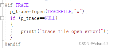
#if TRACE
  p_trace=fopen(TRACEFILE,"w");
  if (p_trace==NULL)
  {
	  printf("trace file open error!");
  }
  DQT_trace = fopen(DQT_file, "w");
  if (DQT_trace == NULL)
  {
      printf("Q_trace file open error!");
  }
  DHT_trace = fopen(DQT_file, "w");
  if (DHT_trace == NULL)
  {
      printf("Q_trace file open error!");
  }
#endif
在DHT函数中打开trace时,表示边运行边写入:
#if TRACE
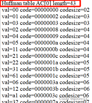
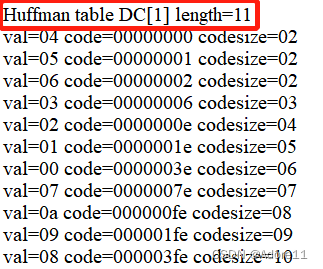
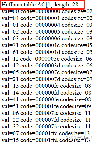
fprintf(p_trace,"Huffman table %s[%d] length=%d\n", (index&0xf0)?"AC":"DC", index&0xf, count);
fflush(p_trace);
fprintf(DHT_trace, "Huffman table %s[%d] length=%d\n", (index & 0xf0) ? "AC" : "DC", index & 0xf, count);
fflush(DHT_trace);
#endif在build_quantization_table函数中将Huffman表打印出来:
#if TRACE
     fprintf(p_trace,"val=%2.2x code=%8.8x codesize=%2.2d\n", val, code, code_size);
	 fflush(p_trace);
     fprintf(DHT_trace, "val=%2.2x code=%8.8x codesize=%2.2d\n", val, code, code_size);
     fflush(DHT_trace);
    #endif
继续打印DQT表:(量化表的标签)
#if TRACE
  fprintf(p_trace,"< DQT marker\n");
  fflush(p_trace);
  fprintf(DQT_trace, "DQT marker:%d\n", qi);
  fflush(DQT_trace);
#endif
build_huffman_table函数中加入如下:打印出 量化表的具体内容:
#if TRACE
for (i=0; i<8; i++) {
for (j=0; j<8; j++) {
fprintf(DQT_trace, "%d\t", ref_table[*zz]);
*qtable++ = ref_table[*zz++] * aanscalefactor[i] * aanscalefactor[j];
}
}
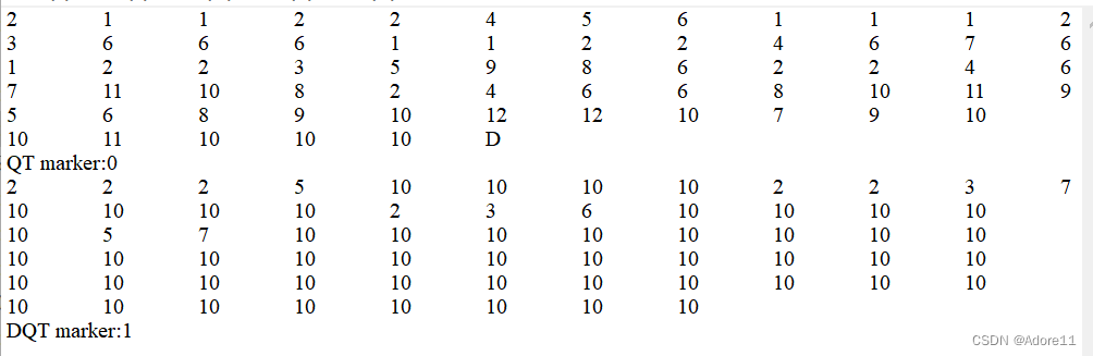
#endif最终得到最后结果:
两张量化表:
可以看出第二张量化表的量化步长更大,最终得到的质量也越不好,根据人眼对色度分量不敏感的特点,我们也能实现推断出第二张图为色度图。
四张huffman表:
亮度分量:
DC系数
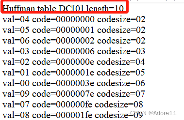
色度分量:
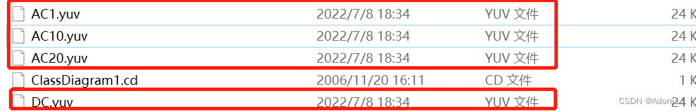
(3)输出DC、AC图像及其概率分布
在tinyjpeg_decode函数中修改~这里注意,DC和AC系数都是指的是DCT变换后,存储DCT变量的数据,DCT[0]即DC图像,DCT[1]~DCT[63]为AC系数:
在decode函数中进行修改:
int tinyjpeg_decode(struct jdec_private *priv, int pixfmt)
{
FILE* DCFile;///DC系数的存储指针
FILE* ACFile_1, * ACFile_10, * ACFile_20;////AC系数的存储指针
DCFile = fopen("DC.yuv", "w");
ACFile_1 = fopen("AC1.yuv", "w");
ACFile_10 = fopen("AC10.yuv", "w");
ACFile_20 = fopen("AC10.yuv", "w");
unsigned char* uvbuf = 128; //将DC系数和AC系数认为是Y分量,uv分量统一设置为128
unsigned char* DCbuf, * ACbuf_1, * ACbuf_10, * ACbuf_20;
int count = 0; //统计Y分量的数量
.......
for (y=0; y < priv->height/ystride_by_mcu; y++)
{
//trace("Decoding row %d\n", y);
priv->plane[0] = priv->components[0] + (y * bytes_per_blocklines[0]);
priv->plane[1] = priv->components[1] + (y * bytes_per_blocklines[1]);
priv->plane[2] = priv->components[2] + (y * bytes_per_blocklines[2]);
for (x=0; x < priv->width; x+=xstride_by_mcu)
{
decode_MCU(priv);
//加入DC,AC的数据接入文件
//DC系数的范围是-512~512,为了使图像能显示,手动+512/4
DCbuf = (unsigned char)((priv->component_infos->DCT[0] + 512) / 4.0);
fwrite(&DCbuf, 1, 1, DCFile);
//AC系数,手动+128,调成正值
ACbuf_1 = (unsigned char)((priv->component_infos->DCT[1] + 128));
fwrite(&ACbuf_1, 1, 1, ACFile_1);
ACbuf_10 = (unsigned char)((priv->component_infos->DCT[10] + 128));
fwrite(&ACbuf_10, 1, 1, ACFile_10);
ACbuf_20 = (unsigned char)((priv->component_infos->DCT[20] + 128));
fwrite(&ACbuf_20, 1, 1, ACFile_20);
convert_to_pixfmt(priv);
priv->plane[0] += bytes_per_mcu[0];
priv->plane[1] += bytes_per_mcu[1];
priv->plane[2] += bytes_per_mcu[2];
if (priv->restarts_to_go>0)
{
priv->restarts_to_go--;
if (priv->restarts_to_go == 0)
{
priv->stream -= (priv->nbits_in_reservoir/8);
resync(priv);
if (find_next_rst_marker(priv) < 0)
return -1;
}
}
}
}
.......
//uv分量写进文件
for (int j = 0; j < count * 0.25 * 2; j++)
{
fwrite(&uvbuf, sizeof(unsigned char), 1, DCFile);
fwrite(&uvbuf, sizeof(unsigned char), 1, ACFile_1);
fwrite(&uvbuf, sizeof(unsigned char), 1, ACbuf_10);
fwrite(&uvbuf, sizeof(unsigned char), 1, ACbuf_20);
}
fclose(DCFile);
fclose(ACFile_1);
fclose(ACbuf_10);
fclose(ACbuf_20);
return 0;
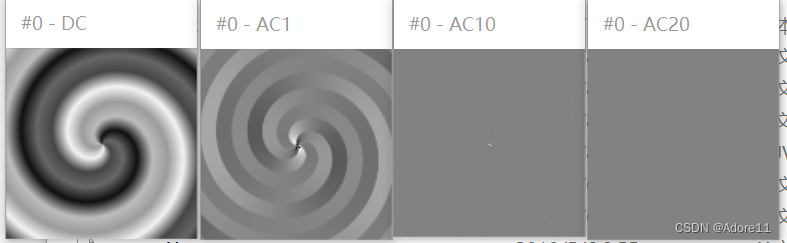
}运行程序,得到两个结果图:
用YUVviewer打开:
统计DC、AC1、AC10、AC20系数的概率分布如下:
| DC系数 | AC1系数 |
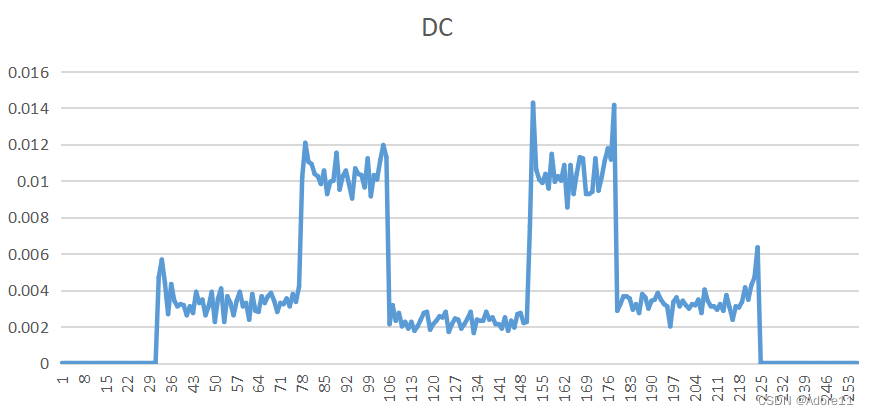 | 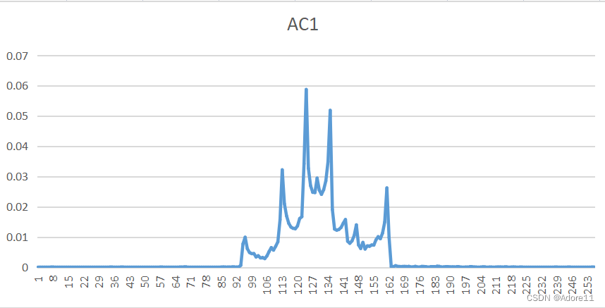 |
| AC10系数 | AC20系数 |
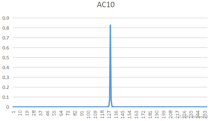 | 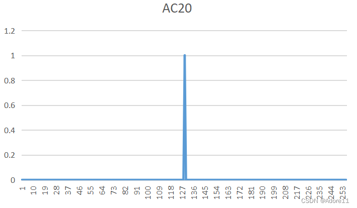 |
通过图片我们可以观察到,DC系数的波动范围大,分布范围广,(具有原图的大部分能量)
AC系数能量较小,且集中于128附近(注意我们刚开始的时候为了保证AC系数为正数,给AC系数+128,现在集中于128证明原来的AC系数集中于0附近。
这也验证了DCT变换后,能量集中于左上角,且主要集中在直流分量上,AC系数能量分布较少。
总结
JPEG编码核心在于DCT变换(变换编码),DCT实现了能量集中、稀疏化和去相关,去除空间冗余,提高了编码效率。DCT变换后,能量大多集中在左上角,低频分量所占的能量大。
但JPEG编码的问题在于:当压缩比较高时,压缩相当于经过了一个低通滤波器,时域体现为于sa函数的卷积,卷积的衰减波纹造成像素间的串扰(容易产生边缘模糊等失真现象)。


 2322
2322

 被折叠的 条评论
为什么被折叠?
被折叠的 条评论
为什么被折叠?
 到【灌水乐园】发言


