


矩阵分解(Matrix Factorization)笔记:非负矩阵分解
非负矩阵分解(NMF)
主要介绍NMF算法原理以及使用sklearn中的封装方法实现该算法,最重要的是理解NMF矩阵分解的实际意义,将其运用到自己的数据分析中!
理论概述
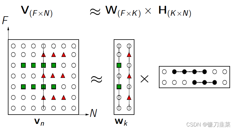
NMF(Non-negative matrix factorization),即对于任意给定的一个非负矩阵
V
=
[
v
1
,
v
2
,
.
.
.
,
v
n
]
∈
R
F
×
N
V=[v_1,v_2,...,v_n]\in \mathcal{R}^{F\times N}
V=[v1,v2,...,vn]∈RF×N,其能够寻找到一个非负矩阵
W
∈
R
F
×
K
W\in \mathcal{R}^{F\times K}
W∈RF×K和一个非负矩阵
H
∈
R
K
×
N
H\in \mathcal{R}^{K\times N}
H∈RK×N,满足条件
V
=
W
×
H
V=W\times H
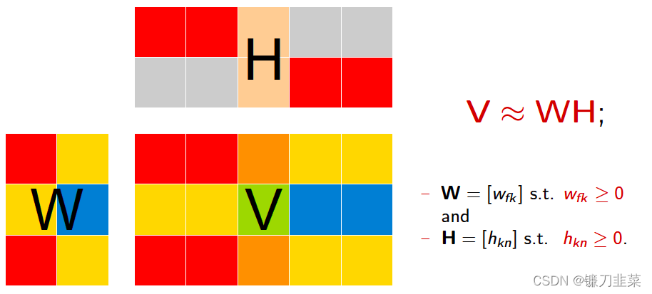
V=W×H,从而将一个非负的矩阵分解为左右两个非负矩阵的乘积。其中,V矩阵中每一列
v
i
v_i
vi代表一个观测(observation),即样本,F为样本维数,N为样本总个数,每一行代表一个特征(feature),
K
<
<
m
i
n
(
F
,
N
)
K<< min(F,N)
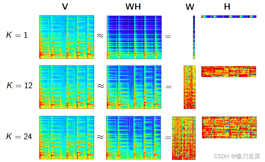
K<<min(F,N);W矩阵称为基矩阵,H矩阵称为系数矩阵或权重矩阵。这时用系数矩阵H代替原始矩阵,就可以实现对原始矩阵进行降维,得到数据特征的降维矩阵,从而减少存储空间。过程如下图所示:
NMF算法采用欧几里得距离的平方来衡量V和
W
×
H
W\times H
W×H之间的重构误差,即最小化以下目标函数:
min
W
,
H
∣
∣
V
−
W
U
∣
∣
F
2
.
s
.
t
.
W
>
=
0
,
H
>
=
0
\min_{W,H}||V-WU||_F^2. s.t.W >=0, H>=0
W,Hmin∣∣V−WU∣∣F2.s.t.W>=0,H>=0
以上目标函数对于联合变量
(
W
,
H
)
(W,H)
(W,H)是非凸的,但是固定单个变量后,目标函数是凸的,可以采用交替乘子法迭代求解。迭代规则如下:
w
i
j
t
+
1
←
w
i
j
t
(
V
H
)
i
j
(
W
H
T
H
)
i
j
w_{ij}^{t+1}\leftarrow w_{ij}^t \frac{(VH)_{ij}}{(WH^TH)_{ij}}
wijt+1←wijt(WHTH)ij(VH)ij
h
i
j
t
+
1
←
h
i
j
t
(
V
T
W
)
i
j
(
H
W
T
W
)
i
j
h_{ij}^{t+1}\leftarrow h_{ij}^t \frac{(V^TW)_{ij}}{(HW^TW)_{ij}}
hijt+1←hijt(HWTW)ij(VTW)ij
为什么分解的矩阵式非负的呢?
- 非负性会引发稀疏
- 非负性会使计算过程进入部分分解
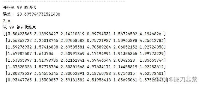
代码如下:
#!/usr/bin/env python
# -*- coding:utf-8 -*-
# @FileName :NMF_demo3.py
# @Time :2022/1/11 16:28
# @Author :PangXZ
import numpy as np
def nmf(X, r, k, e):
'''
参数说明
:param X: 原始矩阵
:param r: 分解的两个非负矩阵的隐变量维度,要远小于原始矩阵的维度
:param k: 迭代次数
:param e: 理想误差
:return: W:基矩阵, H: 系数矩阵
'''
d, n = X.shape
W = np.mat(np.random.rand(d, r))
H = np.mat(np.random.rand(n, r))
x = 1
for x in range(k):
print('---------------------------------------------------')
print('开始第', x, '轮迭代')
X_pre = W * H.T
E = X - X_pre
err = 0.0
for i in range(d):
for j in range(n):
err += E[i, j] * E[i, j]
print('误差:', err)
if err < e:
break
a_w = W * (H.T) * H
b_w = X * H
for p in range(d):
for q in range(r):
if a_w[p, q] != 0:
W[p, q] = W[p, q] * b_w[p, q] / a_w[p, q]
a_h = H * (W.T) * W
b_h = X.T * W
print(r, n)
for c in range(n):
for g in range(r):
if a_h[c, g] != 0:
H[c, g] = H[c, g] * b_h[c, g] / a_h[c, g]
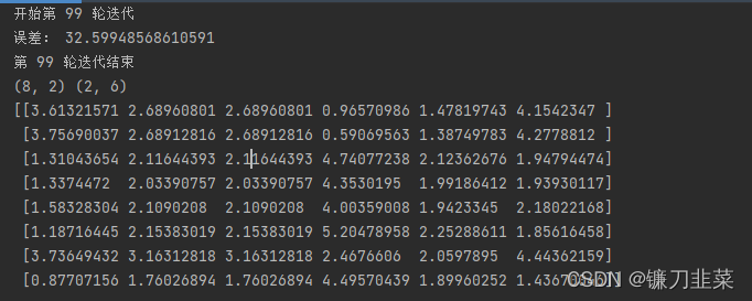
print('第', x, '轮迭代结束')
return W, H
if __name__ == "__main__":
X = [[5, 3, 2, 1, 2, 3],
[4, 2, 2, 1, 1, 5],
[1, 1, 2, 5, 2, 3],
[1, 2, 2, 4, 3, 2],
[2, 1, 5, 4, 1, 1],
[1, 2, 2, 5, 3, 2],
[2, 5, 3, 2, 2, 5],
[2, 1, 2, 5, 1, 1], ]
X = np.mat(X)
W, H = nmf(X, 2, 100, 0.001)
print(W * H.T)
NMF更详尽的原理可以参考Non-negative matrix factorization - Wikipedia,这里主要列出我很关注的损失函数(lossFunction or objective function):
1)squared frobenius norm
arg
min
W
,
H
1
2
∣
∣
A
−
W
H
∣
∣
F
r
o
2
+
α
ρ
∣
∣
W
∣
∣
1
+
α
ρ
∣
∣
H
∣
∣
1
+
α
(
1
−
ρ
)
2
∣
∣
W
∣
∣
F
r
o
2
+
α
(
1
−
ρ
)
2
∣
∣
H
∣
∣
F
r
o
2
\arg \min_{W,H} \frac{1}{2}||A-WH||_{Fro}^2+\alpha\rho ||W||_1+\alpha \rho||H||_1+\frac{\alpha (1-\rho )}{2}||W||_{Fro}^2+\frac{\alpha (1-\rho )}{2}||H||_{Fro}^2
argW,Hmin21∣∣A−WH∣∣Fro2+αρ∣∣W∣∣1+αρ∣∣H∣∣1+2α(1−ρ)∣∣W∣∣Fro2+2α(1−ρ)∣∣H∣∣Fro2
其中:
1
2
∣
∣
A
−
W
H
∣
∣
F
r
o
2
=
1
2
∑
i
,
j
(
A
i
j
−
W
H
i
j
)
2
\frac{1}{2}||A-WH||_{Fro}^2 = \frac{1}{2}\sum_{i,j} (A_{ij}-WH_{ij})^2
21∣∣A−WH∣∣Fro2=21∑i,j(Aij−WHij)2,
α
\alpha
α为L1&L2正则化参数,而
ρ
\rho
ρ为L1正则化占总正则化项的比例。
∣
∣
∗
∣
∣
1
||*||_1
∣∣∗∣∣1为L1范数。
2)Kullback-Leibler (KL)
d
K
L
(
X
,
Y
)
=
∑
i
,
j
(
X
i
,
j
log
(
X
i
j
Y
i
,
j
)
−
X
i
,
j
+
Y
i
,
j
)
d_{KL}(X,Y)=\sum_{i,j}(X_{i,j}\log(\frac{X_{ij}}{Y_{i,j}})-X_{i,j}+Y_{i,j})
dKL(X,Y)=i,j∑(Xi,jlog(Yi,jXij)−Xi,j+Yi,j)
3)Itakura-Saito (IS)
d
I
S
(
X
,
Y
)
=
∑
i
,
j
(
X
i
,
j
Y
i
,
j
−
log
(
X
i
,
j
Y
i
,
j
)
−
1
)
d_{IS}(X,Y)=\sum_{i,j}(\frac{X_{i,j}}{Y_{i,j}}-\log(\frac{X_{i,j}}{Y_{i,j}})-1)
dIS(X,Y)=i,j∑(Yi,jXi,j−log(Yi,jXi,j)−1)
实际上,上面三个公式是beta-divergence family中的三个特殊情况(分别是当
β
=
2
,
1
,
0
\beta = 2, 1, 0
β=2,1,0),其原型是:
d
β
(
X
,
Y
)
=
∑
i
,
j
1
β
(
β
−
1
)
(
X
i
,
j
β
+
(
β
−
1
)
Y
i
,
j
β
−
β
X
i
,
j
Y
i
,
j
β
−
1
)
d_{\beta}(X,Y)=\sum_{i,j} \frac{1}{\beta (\beta-1)}(X_{i,j}^\beta+(\beta-1)Y_{i,j}^\beta-\beta X_{i,j}Y_{i,j}^{\beta-1})
dβ(X,Y)=i,j∑β(β−1)1(Xi,jβ+(β−1)Yi,jβ−βXi,jYi,jβ−1)
其他参考资料:非负矩阵分解(NMF)
代码实现
在sklearn封装了NMF的实现,可以非常方便我们的使用,其实现基本和前面理论部分的实现是一致的,但是注意sklearn中输入数据的格式是(samples, features):
#!/usr/bin/env python
# -*- coding:utf-8 -*-
# @FileName  :NMF_demo.py
# @Time      :2022/1/11 14:26
# @Author    :PangXZ

from sklearn.decomposition import NMF
from sklearn.datasets import load_iris
# Non-Negative Matrix Factorization (NMF).
# Find two non-negative matrices (W, H) whose product approximates the non- negative matrix X.
# This factorization can be used for example for dimensionality reduction, source separation or topic extraction.

if __name__ == "__main__":
    X, _ = load_iris(True)
    # 最重要的参数是n_components, alpha, l1_ratio, solver
    nmf = NMF(n_components=2,    # 样本的数量,如果没有设置n_components,则保留所有特性。
              init=None,         # 用于初始化过程的方法。默认值:None。有效的选项:None/random/nndsvd/nndsvda/nndsvdar
              solver='cd',       # 'cd'/'mu' : “cd”是一个坐标下降求解器。' mu '是一个乘法更新求解器。
              beta_loss='frobenius',  # default ‘frobenius’ 字符串必须是{' frobenius ', ' kullback-leibler ', ' itakura-saito '}。为了使散度最小,测量X和点积WH之间的距离。
              tol=1e-4,          # 停止条件的容忍度。
              max_iter=1000,      # 超时前的最大迭代次数。
              random_state=None, # 用于初始化(当init== ' nndsvdar '或' random '),并在坐标下降。
              alpha=0.,          # 乘正则化项的常数。将它设为0,这样就没有正则化。
              l1_ratio=0.,       # 正则化混合参数,0 <= l1_ratio <= 1。对于l1_ratio = 0,罚分为元素L2罚分(又名Frobenius Norm)。对于l1_ratio = 1,它是元素上的L1惩罚。对于0 < l1_ratio < 1,惩罚为L1和L2的组合。
              verbose=0,         # 是否冗长。
              shuffle=False      # 如果为真,将cd求解器中的坐标顺序随机化。
              )
    print('params:', nmf.get_params()) # 获取构造函数参数的值,也可以nmf.attr得到
    # 核心示例
    nmf.fit(X=X)
    W = nmf.fit_transform(X=X)
    print(W)
    # W = nmf.transform(X=X)
    nmf.inverse_transform(W=W)

    H = nmf.components_ # H矩阵
    print('reconstruction_err_', nmf.reconstruction_err_)  # 损失函数值
    print('n_iter_',nmf.n_iter_)  # 实际迭代次数
注意:
init参数中,nndsvd(默认)更适用于sparse factorization,其变体则适用于dense factorization.solver参数中,如果初始化中产生很多零值,Multiplicative Update (mu)不能很好更新。所以mu一般不和nndsvd使用,而和其变体nndsvda、nndsvdar使用。solver参数中,cd只能优化Frobenius norm函数;而mu可以更新所有损失函数。
示例1
举一个NMF在图像特征提取的应用,来自官方示例:
#!/usr/bin/env python
# -*- coding:utf-8 -*-
# @FileName  :NMF_demo2.py
# @Time      :2022/1/11 15:53
# @Author    :PangXZ
import logging
from time import time

from numpy.random import RandomState
import matplotlib.pyplot as plt

from sklearn.datasets import fetch_olivetti_faces
from sklearn.cluster import MiniBatchKMeans
from sklearn import decomposition

# Display progress logs on stdout
logging.basicConfig(level=logging.INFO, format="%(asctime)s %(levelname)s %(message)s")
n_row, n_col = 2, 3
n_components = n_row * n_col
image_shape = (64, 64)
rng = RandomState(0)

# #############################################################################
# Load faces data
faces, _ = fetch_olivetti_faces(return_X_y=True, shuffle=True, random_state=rng)
n_samples, n_features = faces.shape

# global centering
faces_centered = faces - faces.mean(axis=0)

# local centering
faces_centered -= faces_centered.mean(axis=1).reshape(n_samples, -1)

print("Dataset consists of %d faces" % n_samples)


def plot_gallery(title, images, n_col=n_col, n_row=n_row, cmap=plt.cm.gray):
    plt.figure(figsize=(2.0 * n_col, 2.26 * n_row))
    plt.suptitle(title, size=16)
    for i, comp in enumerate(images):
        plt.subplot(n_row, n_col, i + 1)
        vmax = max(comp.max(), -comp.min())
        plt.imshow(
            comp.reshape(image_shape),
            cmap=cmap,
            interpolation="nearest",
            vmin=-vmax,
            vmax=vmax,
        )
        plt.xticks(())
        plt.yticks(())
    plt.subplots_adjust(0.01, 0.05, 0.99, 0.93, 0.04, 0.0)


# #############################################################################
# List of the different estimators, whether to center and transpose the
# problem, and whether the transformer uses the clustering API.
estimators = [
    (
        "Eigenfaces - PCA using randomized SVD",
        decomposition.PCA(
            n_components=n_components, svd_solver="randomized", whiten=True
        ),
        True,
    ),
    (
        "Non-negative components - NMF",
        decomposition.NMF(n_components=n_components, init="nndsvda", tol=5e-3),
        False,
    ),
    (
        "Independent components - FastICA",
        decomposition.FastICA(n_components=n_components, whiten=True),
        True,
    ),
    (
        "Sparse comp. - MiniBatchSparsePCA",
        decomposition.MiniBatchSparsePCA(
            n_components=n_components,
            alpha=0.8,
            n_iter=100,
            batch_size=3,
            random_state=rng,
        ),
        True,
    ),
    (
        "MiniBatchDictionaryLearning",
        decomposition.MiniBatchDictionaryLearning(
            n_components=15, alpha=0.1, n_iter=50, batch_size=3, random_state=rng
        ),
        True,
    ),
    (
        "Cluster centers - MiniBatchKMeans",
        MiniBatchKMeans(
            n_clusters=n_components,
            tol=1e-3,
            batch_size=20,
            max_iter=50,
            random_state=rng,
        ),
        True,
    ),
    (
        "Factor Analysis components - FA",
        decomposition.FactorAnalysis(n_components=n_components, max_iter=20),
        True,
    ),
]

# #############################################################################
# Plot a sample of the input data

plot_gallery("First centered Olivetti faces", faces_centered[:n_components])

# #############################################################################
# Do the estimation and plot it

for name, estimator, center in estimators:
    print("Extracting the top %d %s..." % (n_components, name))
    t0 = time()
    data = faces
    if center:
        data = faces_centered
    estimator.fit(data)
    train_time = time() - t0
    print("done in %0.3fs" % train_time)
    if hasattr(estimator, "cluster_centers_"):
        components_ = estimator.cluster_centers_
    else:
        components_ = estimator.components_

    # Plot an image representing the pixelwise variance provided by the
    # estimator e.g its noise_variance_ attribute. The Eigenfaces estimator,
    # via the PCA decomposition, also provides a scalar noise_variance_
    # (the mean of pixelwise variance) that cannot be displayed as an image
    # so we skip it.
    if (
            hasattr(estimator, "noise_variance_") and estimator.noise_variance_.ndim > 0
    ):  # Skip the Eigenfaces case
        plot_gallery(
            "Pixelwise variance",
            estimator.noise_variance_.reshape(1, -1),
            n_col=1,
            n_row=1,
        )
    plot_gallery(
        "%s - Train time %.1fs" % (name, train_time), components_[:n_components]
    )

plt.show()

# #############################################################################
# Various positivity constraints applied to dictionary learning.
estimators = [
    (
        "Dictionary learning",
        decomposition.MiniBatchDictionaryLearning(
            n_components=15, alpha=0.1, n_iter=50, batch_size=3, random_state=rng
        ),
        True,
    ),
    (
        "Dictionary learning - positive dictionary",
        decomposition.MiniBatchDictionaryLearning(
            n_components=15,
            alpha=0.1,
            n_iter=50,
            batch_size=3,
            random_state=rng,
            positive_dict=True,
        ),
        True,
    ),
    (
        "Dictionary learning - positive code",
        decomposition.MiniBatchDictionaryLearning(
            n_components=15,
            alpha=0.1,
            n_iter=50,
            batch_size=3,
            fit_algorithm="cd",
            random_state=rng,
            positive_code=True,
        ),
        True,
    ),
    (
        "Dictionary learning - positive dictionary & code",
        decomposition.MiniBatchDictionaryLearning(
            n_components=15,
            alpha=0.1,
            n_iter=50,
            batch_size=3,
            fit_algorithm="cd",
            random_state=rng,
            positive_dict=True,
            positive_code=True,
        ),
        True,
    ),
]

# #############################################################################
# Plot a sample of the input data

plot_gallery(
    "First centered Olivetti faces", faces_centered[:n_components], cmap=plt.cm.RdBu
)

# #############################################################################
# Do the estimation and plot it

for name, estimator, center in estimators:
    print("Extracting the top %d %s..." % (n_components, name))
    t0 = time()
    data = faces
    if center:
        data = faces_centered
    estimator.fit(data)
    train_time = time() - t0
    print("done in %0.3fs" % train_time)
    components_ = estimator.components_
    plot_gallery(name, components_[:n_components], cmap=plt.cm.RdBu)

plt.show()
NMF最早由科学家D.D.Lee和H.S.Seung提出的一种非负矩阵分解方法,并在Nature发表文章《Learning the parts of objects by non-negative matrix factorization》。随后也有了很多NMF变体,应用也越发广泛,包括文本降维、话题提取、图像处理等。有兴趣的同学也可以参考Nimfa。
import nimfa

if __name__ == "__main__":
    V = nimfa.examples.medulloblastoma.read(normalize=True)
    lsnmf = nimfa.Lsnmf(V, seed='random_vcol', rank=50, max_iter=100)
    lsnmf_fit = lsnmf()
    print('Rss: %5.4f' % lsnmf_fit.fit.rss())
    print('Evar: %5.4f' % lsnmf_fit.fit.evar())
    print('K-L divergence: %5.4f' % lsnmf_fit.distance(metric='kl'))
    print('Sparseness, W: %5.4f, H: %5.4f' % lsnmf_fit.fit.sparseness())
相关问题
如何选择K值
对于一个适当的K选择在于分解的时候很重要,其中不同的K对于不同模型情况如下:
- 数据拟合:K越大那么对于数据拟合更好
- 模型复杂性:一个更小的K模型更简单(易于预测、少输入参数等)
解不唯一
对于 V = W H ; W > = 0 , H > = 0 V=WH;W>=0,H>=0 V=WH;W>=0,H>=0,那么任意一个矩阵Q有 W Q > = 0 , Q − 1 H > = 0 WQ>=0, Q^{-1}H>=0 WQ>=0,Q−1H>=0,这就提供了一个可以替换的因子 V = W H = ( W Q ) ( Q − 1 H ) V=WH=(WQ)(Q^{-1}H) V=WH=(WQ)(Q−1H),特殊情况下,Q可以为任意非负广义置换矩阵。虽然解不唯一,但是一般情况下解不唯一仅仅是基向量 W k W_k Wk的缩放和转置,也就是换来换去还是它自己本身。
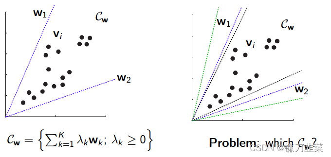
几何意义
NMF假设数据是由W所产生的一个凸角 C w C_w Cw,对于 C w C_w Cw来说就很郁闷啦,因为可以有很多个不用的 w i w_i wi来决定,因此很难确定到底是哪个 C w C_w Cw。那,怎么解决这个问题呢,学数学的人知道应该引入约束式来限制 w i w_i wi的选择。对于怎么选择约束,业界已经出现了很多种方法:
- 稀疏约束(e.g., Hoyer, 2004; Eggert and Korner, 2004);
- 形状约束
- 对 h k h_k hk的空间或时间约束:activations are smooth (Virtanen, 2007; Jia and Qian, 2009; Essid and Fevotte, 2013)
- 跨模态对应约束(Seichepine et al., 2013; Liu et al., 2013; Yilmaz etal., 2011)
- 几何约束,例如,选择特殊的角点
C
w
C_w
Cw(Klingenberg et al.,2009; Essid, 2012)
应用概述
在众多应用中,NMF能被用于发现数据库中的图像特征,便于快速自动识别应用;能够发现文档的语义相关度,用于信息自动索引和提取;能够在DNA阵列分析中识别基因等等。我们将对此作一些大致的描述。但是最有效的就是图像处理领域,是图像处理的数据降维和特征提取的一种有效方法。
约束非负矩阵分解(CNMF)
约束非负矩阵分解(CNMF)算法,该算法将标签信息作为附加的硬约束,使得具有相同类标签信息的数据在新的低维空间中仍然保持一致。但是,CNMF算法对于无标签数据样本没有任何约束,因此在很少的标签信息时它的性能受限,并且对于类中只有一个样本有标签的情形,CNMF算法中构建的约束矩阵将退化为单位矩阵,失去其意义。
算法讲解
CNMF算法假设数据集X中共包含c类样本,其中前
l
l
l个样本
x
1
,
.
.
.
,
x
l
x_1,...,x_l
x1,...,xl标签信息已知,其余
n
−
l
n-l
n−l个样本,即
x
l
+
1
,
.
.
.
,
x
n
x_{l+1},...,x_n
xl+1,...,xn标签信息未知。首先对于前
l
l
l个有标签的样本,定义指示矩阵
C
∈
R
l
×
c
C\in \mathcal{R}^{l\times c}
C∈Rl×c,如下:
c
i
j
=
{
1
,
如果
x
i
∈
第
j
类
0
其他
c_{ij}=\left\{\begin{matrix} 1, & 如果x_i\in第j类\\ 0 & 其他 \end{matrix}\right.
cij={1,0如果xi∈第j类其他
然后关于所有样本,定义样本约束矩阵
A
∈
R
n
×
(
n
+
c
−
l
)
A\in \mathcal{R}^{n \times (n+c-l)}
A∈Rn×(n+c−l):
A
=
(
C
0
0
I
)
A=\begin{pmatrix} C & 0\\ 0 & I \end{pmatrix}
A=(C00I)
其中,
I
∈
R
(
n
−
l
)
×
(
n
−
l
)
I\in \mathcal{R}^{(n-l)\times(n-l)}
I∈R(n−l)×(n−l)是单位矩阵,
CNMF算法引入辅助矩阵
Z
∈
R
(
n
+
c
−
l
)
Z\in \mathcal{R}^{(n+c-l)}
Z∈R(n+c−l)将以上样本的约束矩阵嵌入目标函数中,使得V中的属于同一类的样本映射为同一点,令
V
=
A
Z
V=AZ
V=AZ,即最小化以下目标函数:
min
U
,
V
∣
∣
X
−
U
(
A
Z
)
T
∣
∣
F
2
,
s
.
t
.
U
>
=
0
,
V
>
=
0
\min_{U,V}{||X-U(AZ)^T||_F^2, s.t.U>=0, V>=0}
minU,V∣∣X−U(AZ)T∣∣F2,s.t.U>=0,V>=0
综上,采用交替迭代法进行求解,迭代规则如下:
u
i
j
(
t
+
1
)
←
u
i
j
(
t
)
(
X
A
Z
)
i
j
(
U
Z
T
A
T
A
Z
)
i
j
u_{ij}^{(t+1)}\leftarrow u_{ij}^{(t)}\frac{(XAZ)_{ij}}{(UZ^TA^TAZ)_{ij}}
uij(t+1)←uij(t)(UZTATAZ)ij(XAZ)ij
z
i
j
(
t
+
1
)
←
z
i
j
(
t
)
(
A
T
X
T
U
)
i
j
(
A
T
A
Z
U
T
U
)
i
j
z_{ij}^{(t+1)}\leftarrow z_{ij}^{(t)}\frac{(A^TX^TU)_{ij}}{(A^TAZU^TU)_{ij}}
zij(t+1)←zij(t)(ATAZUTU)ij(ATXTU)ij
简单地说,就是在原有的NMF的基础上增加了一个标签信息的硬约束。把原本的V改成了AZ,其中A就是表示样本标签的一个矩阵。
代码实现
#!/usr/bin/env python
# -*- coding:utf-8 -*-
# @FileName  :CNMF.py
# @Time      :2022/1/11 19:43
# @Author    :PangXZ
import numpy as np


def cnmf(X, C, r, k, e):
    '''
    参数描述
    :param X: 原始矩阵,维度为d*n
    :param C: 有标签样本指示矩阵,维度为l*c (l:有标签的样本的数量,c:类别数量)
    :param r: 分解的两个非负矩阵的隐变量维度,要远小于原始矩阵的维度
    :param k: 迭代次数
    :param e: 理想误差
    :return: U:基矩阵 V:系数矩阵
    '''
    d, n = X.shape
    l, c = C.shape

    # 计算A矩阵
    I = np.mat(np.identity(n - l))
    A = np.zeros((n, n + c - l))

    for i in range(l):
        for j in range(c):
            A[i, j] = C[i, j]
    for q in range(n - l):
        A[l + q, c + q] = I[q, q]
    A = np.mat(A)
    U = np.mat(np.random.rand(d, r))
    Z = np.mat(np.random.rand(n + c - l, r))

    x = 1
    for x in range(k):
        print('-------------------------------------------------')
        print('开始第', x, '轮迭代')
        X_pre = U * (A * Z).T
        E = X - X_pre
        # print(E)
        err = 0.0
        for i in range(d):
            for j in range(n):
                err += E[i, j] * E[i, j]
        print('误差:', err)

        if err < e:
            break
        # update U
        a_u = U * Z.T * A.T * A * Z
        b_u = X * A * Z
        for i in range(d):
            for j in range(r):
                if a_u[i, j] != 0:
                    U[i, j] = U[i, j] * b_u[i, j] / a_u[i, j]
        # print(U)

        # update Z
        # print(Z.shape,n,r)
        a_z = A.T * A * Z * U.T * U
        b_z = A.T * X.T * U
        for i in range(n + c - l):
            for j in range(r):
                if a_z[i, j] != 0:
                    Z[i, j] = Z[i, j] * b_z[i, j] / a_z[i, j]
        # print(Z)
        print('第', x, '轮迭代结束')

    V = (A * Z).T
    return U, V


if __name__ == "__main__":
    X = [[5, 3, 2, 1, 2, 3],
         [4, 2, 2, 1, 1, 5],
         [1, 1, 2, 5, 2, 3],
         [1, 2, 2, 4, 3, 2],
         [2, 1, 5, 4, 1, 1],
         [1, 2, 2, 5, 3, 2],
         [2, 5, 3, 2, 2, 5],
         [2, 1, 2, 5, 1, 1], ]  # 8*6,6个样本
    X = np.mat(X)
    C = [[0, 0, 1],
         [0, 1, 0],
         [0, 1, 0],
         [1, 0, 0], ]  # 4*3,假设有4个样本有标签,总共有三类标签
    C = np.mat(C)
    U, V = cnmf(X, C, 2, 100, 0.01)
    print(U.shape, V.shape)
    print(U * V)
通过对比误差,发现NMF比CNMF的误差更小。
参考资料
- https://blog.youkuaiyun.com/jeffery0207/article/details/84348117
- https://www.jianshu.com/p/49a5bd0d422d
- https://blog.youkuaiyun.com/qq_26225295/article/details/51211529


笔记:非负矩阵分解&spm=1001.2101.3001.5002&articleId=121791752&d=1&t=3&u=c9a15c90da5643c29ed3706a19f190f6)
 1910
1910


 到【灌水乐园】发言


