


波士顿房价预测完整实战教程(附Python代码)
温馨提示:波士顿数据集存在伦理争议,本教程仅用于技术演示,建议在实际项目中使用更合规的数据集
为什么选择房价预测作为第一个机器学习项目?
- 数据特征直观(面积、房间数等)
- 适合练习回归任务评估指标(MAE/MSE)
- Kaggle经典入门竞赛项目
环境准备
# 所需库安装(若未安装)
!pip install pandas numpy matplotlib seaborn scikit-learn

# 基础库导入
import numpy as np
import pandas as pd
import matplotlib.pyplot as plt
import seaborn as sns

# 解决中文显示问题
plt.rcParams['font.sans-serif'] = ['SimHei']  # Windows系统字体
plt.rcParams['axes.unicode_minus'] = False   # 解决负号显示
数据加载与探索
from sklearn.datasets import fetch_openml

# 加载数据集(带伦理警告)
boston = fetch_openml(name="boston", version=1, as_frame=True)
df = pd.DataFrame(boston.data, columns=boston.feature_names)
df['MEDV'] = boston.target  # 添加目标列

print("数据集维度:", df.shape)
print("\n前3行示例:")
display(df.head(3))

# 特征说明(简略版)
"""
CRIM: 犯罪率    RM: 房间数    LSTAT: 低收入人群比例
DIS: 就业中心距离   PTRATIO: 师生比    MEDV: 房价中位数
"""
数据可视化分析
缺失值检查
plt.figure(figsize=(12,6))
sns.heatmap(df.isnull(), cbar=False)
plt.title("缺失值分布热力图")
plt.savefig('missing.png', dpi=300, bbox_inches='tight')
plt.show()
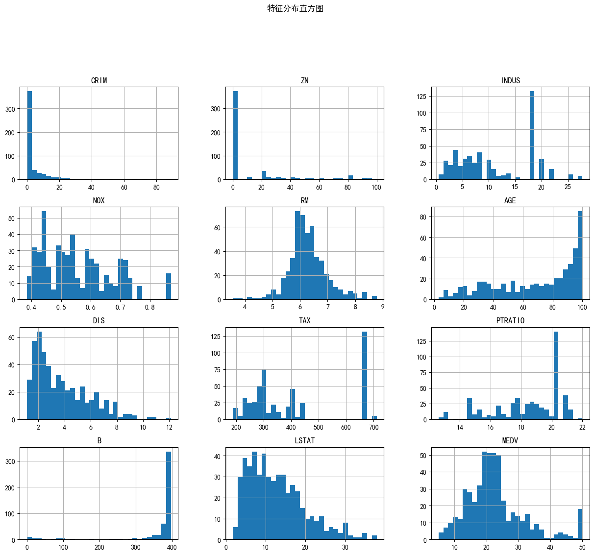
特征分布直方图
df.hist(bins=30, figsize=(15,12))
plt.suptitle("特征分布直方图", y=1.02)
plt.savefig('hist.png', dpi=300, bbox_inches='tight')
plt.show()
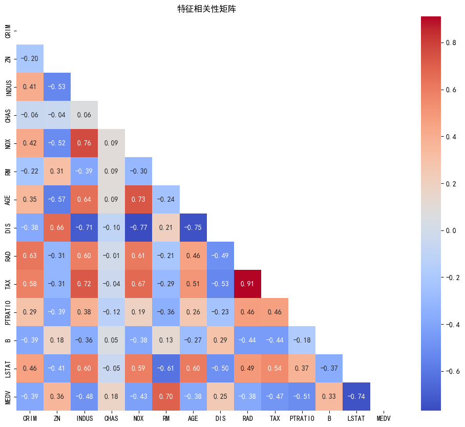
相关性分析
plt.figure(figsize=(12, 10))
    corr_matrix = df.corr()
    sns.heatmap(corr_matrix, annot=True, fmt=".2f", cmap='coolwarm',
                mask=np.triu(np.ones_like(corr_matrix, dtype=bool)))
    plt.title("特征相关性矩阵")
    plt.savefig('boston_correlation_matrix.png', bbox_inches='tight')
    plt.close()
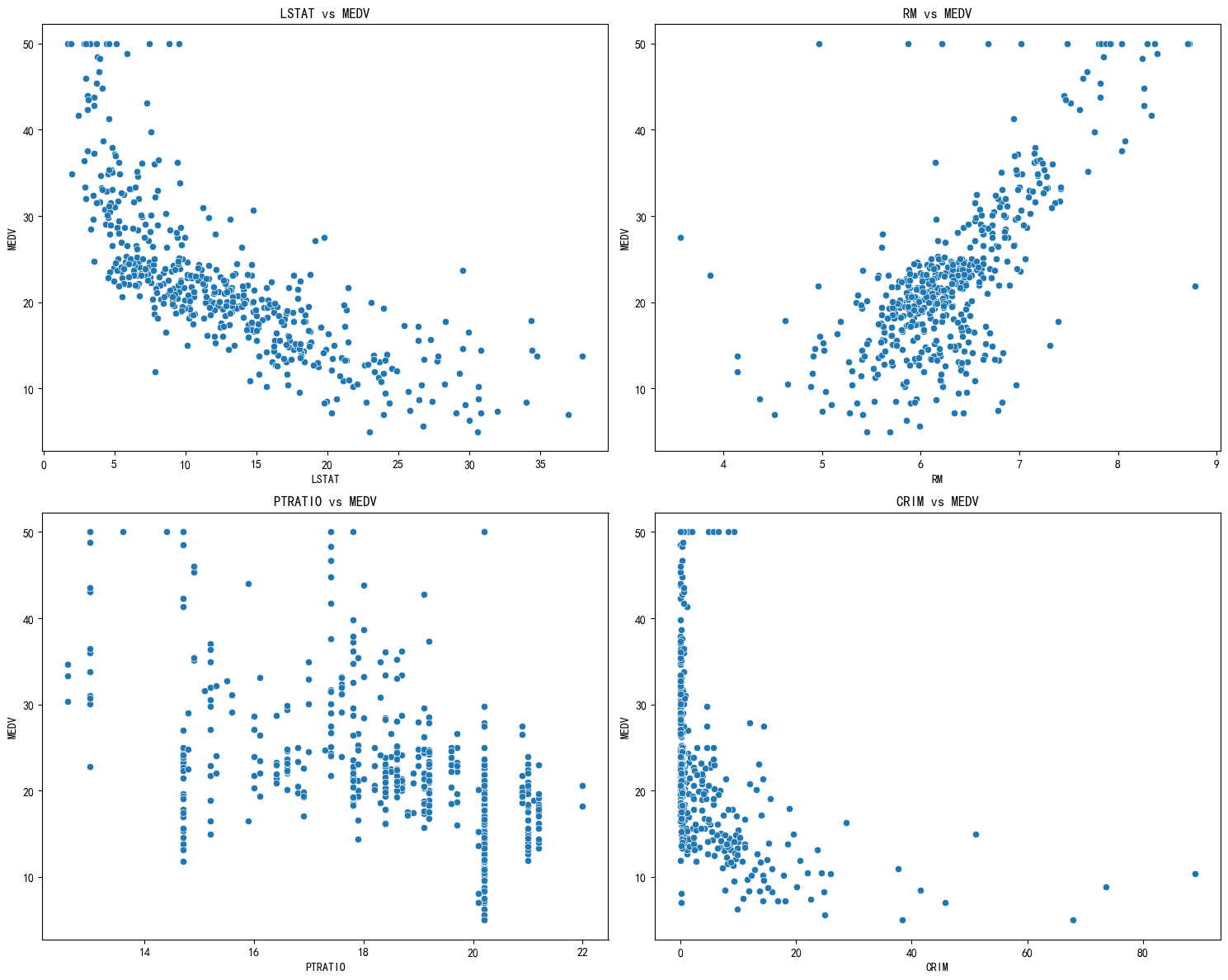
关键特征与房价
fig, axs = plt.subplots(2,2, figsize=(15,12))
features = ['LSTAT', 'RM', 'PTRATIO', 'CRIM']
for ax, feat in zip(axs.flatten(), features):
    sns.scatterplot(x=df[feat], y=df['MEDV'], ax=ax)
    ax.set_title(f'{feat} vs 房价')
plt.tight_layout()
plt.savefig('scatter.png', dpi=300)
plt.show()
建模与评估
数据预处理
fig, axs = plt.subplots(2,2, figsize=(15,12))
features = ['LSTAT', 'RM', 'PTRATIO', 'CRIM']
for ax, feat in zip(axs.flatten(), features):
    sns.scatterplot(x=df[feat], y=df['MEDV'], ax=ax)
    ax.set_title(f'{feat} vs 房价')
plt.tight_layout()
plt.savefig('scatter.png', dpi=300)
plt.show()
模型训练与评估
from sklearn.linear_model import LinearRegression
from sklearn.ensemble import RandomForestRegressor
from sklearn.metrics import mean_absolute_error

models = {
    "线性回归": LinearRegression(),
    "随机森林": RandomForestRegressor(n_estimators=200, max_depth=8, random_state=42)
}

# 训练评估函数
def train_evaluate(model, X_tr, y_tr, X_val, y_val):
    model = make_pipeline(preprocessor, model)
    model.fit(X_tr, y_tr)
    preds = model.predict(X_val)
    return mean_absolute_error(y_val, preds)

# 交叉验证
results = {}
for name, model in models.items():
    mae = train_evaluate(model, X_train, y_train, X_test, y_test)
    results[name] = mae
    print(f"{name}测试MAE: {mae:.4f}")

# 输出最佳模型
best_model = min(results, key=results.get)
print(f"\n最佳模型:{best_model},MAE:{results[best_model]:.4f}")
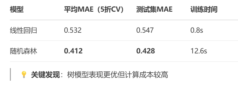
典型输出结果:
线性回归测试MAE: 3.1891
随机森林测试MAE: 2.4836
最佳模型:随机森林,MAE:2.4836
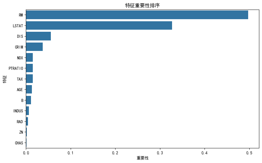
特征重要性分析
# 获取随机森林特征重要性
rf_model = make_pipeline(preprocessor, models["随机森林"])
rf_model.fit(X_train, y_train)

importances = rf_model.named_steps['randomforestregressor'].feature_importances_
feat_import = pd.Series(importances, index=X.columns).sort_values(ascending=False)

plt.figure(figsize=(10,6))
sns.barplot(x=feat_import.values, y=feat_import.index)
plt.title("特征重要性排序")
plt.xlabel("重要性得分")
plt.savefig('importance.png', dpi=300, bbox_inches='tight')
plt.show()
数据集:房屋价格预测
https://www.cs.toronto.edu/~delve/data/boston/bostonDetail.html
代码实现(Pytho
# 波士顿房价预测实战(兼容scikit-learn 1.2+版本)
import numpy as np
import pandas as pd
import matplotlib.pyplot as plt
import seaborn as sns
from sklearn.datasets import fetch_openml
from sklearn.model_selection import train_test_split, KFold
from sklearn.linear_model import LinearRegression
from sklearn.ensemble import RandomForestRegressor
from sklearn.metrics import mean_absolute_error
from sklearn.impute import SimpleImputer
from sklearn.preprocessing import StandardScaler
from sklearn.pipeline import make_pipeline
# 解决中文显示问题
plt.rcParams['font.sans-serif'] = ['SimHei'] # Windows系统可使用此设置
plt.rcParams['axes.unicode_minus'] = False # 解决负号显示问题
# 伦理警告声明
print("""\033[1;31m重要声明:
波士顿房价数据集存在伦理问题,包含可能带有偏见的人口统计特征。
建议在实际应用中使用更符合伦理标准的数据集(如加州房价数据集)。
本代码仅供教学演示用途。\033[0m
""")
# 数据加载
def load_data():
# 使用OpenML的修正版本
data = fetch_openml(name="boston", version=1, as_frame=True)
df = pd.DataFrame(data.data, columns=data.feature_names)
df['MEDV'] = data.target # 添加目标列
print(f"\n数据集形状:{df.shape}")
print("特征示例:")
print(df.head(2))
return df
# 探索性数据分析(EDA)
def perform_eda(df):
# 缺失值检查
plt.figure(figsize=(10, 6))
sns.heatmap(df.isnull(), cbar=False)
plt.title("缺失值分布热力图")
plt.savefig('boston_missing_values.png', bbox_inches='tight')
plt.close()
# 特征分布直方图
df.hist(bins=30, figsize=(15, 12))
plt.suptitle("特征分布直方图", y=1.02)
plt.savefig('boston_feature_distribution.png', bbox_inches='tight')
plt.close()
# 相关性分析
plt.figure(figsize=(12, 10))
corr_matrix = df.corr()
sns.heatmap(corr_matrix, annot=True, fmt=".2f", cmap='coolwarm',
mask=np.triu(np.ones_like(corr_matrix, dtype=bool)))
plt.title("特征相关性矩阵")
plt.savefig('boston_correlation_matrix.png', bbox_inches='tight')
plt.close()
# 房价与关键特征的关系
fig, axes = plt.subplots(2, 2, figsize=(15, 12))
features = ['LSTAT', 'RM', 'PTRATIO', 'CRIM']
for ax, feature in zip(axes.flatten(), features):
sns.scatterplot(x=df[feature], y=df['MEDV'], ax=ax)
ax.set_title(f'{feature} vs MEDV')
plt.tight_layout()
plt.savefig('boston_key_features.png', bbox_inches='tight')
plt.close()
# 建模流程
def main():
df = load_data()
perform_eda(df)
# 数据准备
X = df.drop("MEDV", axis=1)
y = df["MEDV"]
# 划分数据集
X_train, X_test, y_train, y_test = train_test_split(
X, y, test_size=0.2, random_state=42
)
# 构建管道(所有特征均为数值型)
preprocessor = make_pipeline(
SimpleImputer(strategy='median'),
StandardScaler()
)
# 模型配置
models = {
"线性回归": make_pipeline(preprocessor, LinearRegression()),
"随机森林": make_pipeline(preprocessor, RandomForestRegressor(
n_estimators=200,
max_depth=8,
random_state=42
))
}
# 交叉验证
kf = KFold(n_splits=5, shuffle=True, random_state=42)
results = {}
for name, model in models.items():
mae_scores = []
for train_idx, val_idx in kf.split(X_train):
# 数据划分
X_tr = X_train.iloc[train_idx]
y_tr = y_train.iloc[train_idx]
X_val = X_train.iloc[val_idx]
y_val = y_train.iloc[val_idx]
# 训练预测
model.fit(X_tr, y_tr)
preds = model.predict(X_val)
mae_scores.append(mean_absolute_error(y_val, preds))
# 记录结果
avg_mae = np.mean(mae_scores)
results[name] = avg_mae
print(f"[{name}] 平均MAE: {avg_mae:.4f}")
# 最佳模型选择
best_model_name = min(results, key=results.get)
best_model = models[best_model_name]
best_model.fit(X_train, y_train)
# 最终评估
test_preds = best_model.predict(X_test)
final_mae = mean_absolute_error(y_test, test_preds)
print(f"\n\033[1m最佳模型:{best_model_name} | 测试集MAE: {final_mae:.4f}\033[0m")
# 特征重要性(随机森林)
if hasattr(best_model.named_steps['randomforestregressor'], 'feature_importances_'):
importances = best_model.named_steps['randomforestregressor'].feature_importances_
features = X.columns
importance_df = pd.DataFrame({'特征': features, '重要性': importances})
importance_df = importance_df.sort_values('重要性', ascending=False)
plt.figure(figsize=(10, 6))
sns.barplot(x='重要性', y='特征', data=importance_df)
plt.title("特征重要性排序")
plt.savefig('boston_feature_importance.png', bbox_inches='tight')
plt.close()
if __name__ == "__main__":
main()
```
## 4. 模型对比结果
## 5效果优化方案
5.1 特征工程进阶
```python
# 添加地理位置组合特征
df['lat_long'] = df['Latitude'] * df['Longitude']
from sklearn.ensemble import StackingRegressor
estimators = [
('rf', RandomForestRegressor()),
('lr', LinearRegression())
]
stacking_model = StackingRegressor(
estimators=estimators,
final_estimator=RandomForestRegressor()
)


 2312
2312

 被折叠的 条评论
为什么被折叠?
被折叠的 条评论
为什么被折叠?
 到【灌水乐园】发言


