训练误差or测试误差与特征个数之间的关系--基于R语言实现

a 生成数据集，数据由$Y=X\beta +ϵ$产生，其中$p=20，n=1000$

#way1
set.seed(1)
p = 20
n = 1000
x = matrix(rnorm(n*p), n, p)
B = rnorm(p)
B[3] = 0
B[4] = 0
B[9] = 0
B[19] = 0
B[10] = 0
eps = rnorm(p)
y = x %*% B + eps#%*%为矩阵乘法

#way2
set.seed(1)
a=rnorm(20*1000)
x=matrix(a,1000,20)
eps=rnorm(1000)
beta=c(1,1,0,0,5.5,2,5,0,4,0,1.5,11,10.5,3.3,2.8,0,9,0,2,6.6)
y=x%*%beta+eps#%*%为矩阵乘法

其中部分元素为0。

b 划分数据为训练集和测试集

#way1
train = sample(seq(1000), 100, replace = FALSE)
y.train = y[train,]
y.test = y[-train,]
x.train = x[train,]
x.test = x[-train,]

#way2
train=sample(1:1000,100,rep=F)
test=(-train)

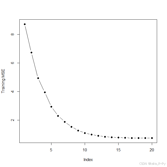
c 训练集MSE分析

#way1
library(leaps)
regfit.full = regsubsets(y~., data=data.frame(x=x.train, y=y.train), nvmax=p)
val.errors = rep(NA, p)
x_cols = colnames(x, do.NULL=FALSE, prefix="x.")
for (i in 1:p) {
  coefi = coef(regfit.full, id=i)
  pred = as.matrix(x.train[, x_cols %in% names(coefi)]) %*% coefi[names(coefi) %in% x_cols]
  val.errors[i] = mean((y.train - pred)^2)
}
plot(val.errors, ylab="Training MSE", pch=19, type="b")

#way2
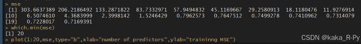
library(leaps)
d=data.frame(y,x)
fit1=regsubsets(y~.,data=d,subset=train,nvmax=20)
s1=summary(fit1)
mse=(s1$rss)/100
mse
which.min(mse)
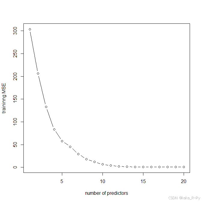
plot(1:20,mse,type="b",xlab="number of predictors",ylab="traininng MSE")

> d=data.frame(y,x)
> fit1=regsubsets(y~.,data=d,subset=train,nvmax=20)
> s1=summary(fit1)
> s1
Subset selection object
Call: regsubsets.formula(y ~ ., data = d, subset = train, nvmax = 20)
20 Variables  (and intercept)
    Forced in Forced out
X1      FALSE      FALSE
X2      FALSE      FALSE
X3      FALSE      FALSE
X4      FALSE      FALSE
X5      FALSE      FALSE
X6      FALSE      FALSE
X7      FALSE      FALSE
X8      FALSE      FALSE
X9      FALSE      FALSE
X10     FALSE      FALSE
X11     FALSE      FALSE
X12     FALSE      FALSE
X13     FALSE      FALSE
X14     FALSE      FALSE
X15     FALSE      FALSE
X16     FALSE      FALSE
X17     FALSE      FALSE
X18     FALSE      FALSE
X19     FALSE      FALSE
X20     FALSE      FALSE
1 subsets of each size up to 20
Selection Algorithm: exhaustive
          X1  X2  X3  X4  X5  X6  X7  X8  X9  X10 X11 X12 X13 X14 X15 X16 X17 X18 X19 X20
1  ( 1 )  " " " " " " " " " " " " " " " " " " " " " " "*" " " " " " " " " " " " " " " " "
2  ( 1 )  " " " " " " " " " " " " " " " " " " " " " " "*" " " " " " " " " "*" " " " " " "
3  ( 1 )  " " " " " " " " " " " " " " " " " " " " " " "*" "*" " " " " " " "*" " " " " " "
4  ( 1 )  " " " " " " " " " " " " " " " " " " " " " " "*" "*" " " " " " " "*" " " " " "*"
5  ( 1 )  " " " " " " " " "*" " " " " " " " " " " " " "*" "*" " " " " " " "*" " " " " "*"
6  ( 1 )  " " " " " " " " "*" " " "*" " " " " " " " " "*" "*" " " " " " " "*" " " " " "*"
7  ( 1 )  " " " " " " " " "*" " " "*" " " "*" " " " " "*" "*" " " " " " " "*" " " " " "*"
8  ( 1 )  " " " " " " " " "*" " " "*" " " "*" " " " " "*" "*" "*" " " " " "*" " " " " "*"
9  ( 1 )  " " " " " " " " "*" " " "*" " " "*" " " " " "*" "*" "*" "*" " " "*" " " " " "*"
10  ( 1 ) " " " " " " " " "*" " " "*" " " "*" " " " " "*" "*" "*" "*" " " "*" " " "*" "*"
11  ( 1 ) " " " " " " " " "*" "*" "*" " " "*" " " " " "*" "*" "*" "*" " " "*" " " "*" "*"
12  ( 1 ) " " " " " " " " "*" "*" "*" " " "*" " " "*" "*" "*" "*" "*" " " "*" " " "*" "*"
13  ( 1 ) " " "*" " " " " "*" "*" "*" " " "*" " " "*" "*" "*" "*" "*" " " "*" " " "*" "*"
14  ( 1 ) "*" "*" " " " " "*" "*" "*" " " "*" " " "*" "*" "*" "*" "*" " " "*" " " "*" "*"
15  ( 1 ) "*" "*" " " " " "*" "*" "*" "*" "*" " " "*" "*" "*" "*" "*" " " "*" " " "*" "*"
16  ( 1 ) "*" "*" " " " " "*" "*" "*" "*" "*" " " "*" "*" "*" "*" "*" " " "*" "*" "*" "*"
17  ( 1 ) "*" "*" "*" " " "*" "*" "*" "*" "*" " " "*" "*" "*" "*" "*" " " "*" "*" "*" "*"
18  ( 1 ) "*" "*" "*" "*" "*" "*" "*" "*" "*" " " "*" "*" "*" "*" "*" " " "*" "*" "*" "*"
19  ( 1 ) "*" "*" " " "*" "*" "*" "*" "*" "*" "*" "*" "*" "*" "*" "*" "*" "*" "*" "*" "*"
20  ( 1 ) "*" "*" "*" "*" "*" "*" "*" "*" "*" "*" "*" "*" "*" "*" "*" "*" "*" "*" "*" "*"

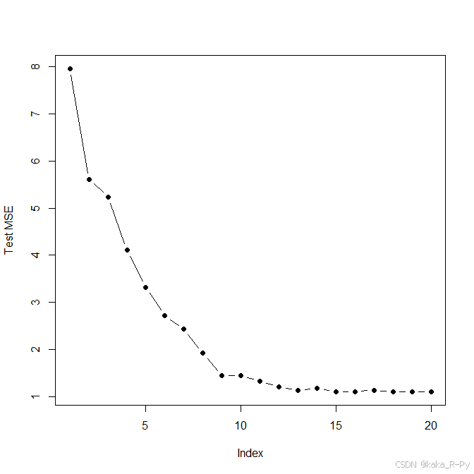
d 测试集MSE分析

#way1
val.errors = rep(NA, p)
for (i in 1:p) {
  coefi = coef(regfit.full, id=i)
  pred = as.matrix(x.test[, x_cols %in% names(coefi)]) %*% coefi[names(coefi) %in% x_cols]#测试集的Y
  val.errors[i] = mean((y.test - pred)^2)#计算MSE
}
plot(val.errors, ylab="Test MSE", pch=19, type="b")

#way2
xmat=model.matrix(y~.,data=d)
mse1=rep(NA,20)
for(i in 1:20){
  pred=xmat[test,][,names(coefficients(
    fit1,id=i))]%*%coefficients(fit1,id=i)
  mse1[i]=mean((pred-y[test])^2)
}
mse1
plot(1:20,mse1,type="b",xlab="model size",ylab="test MSE")

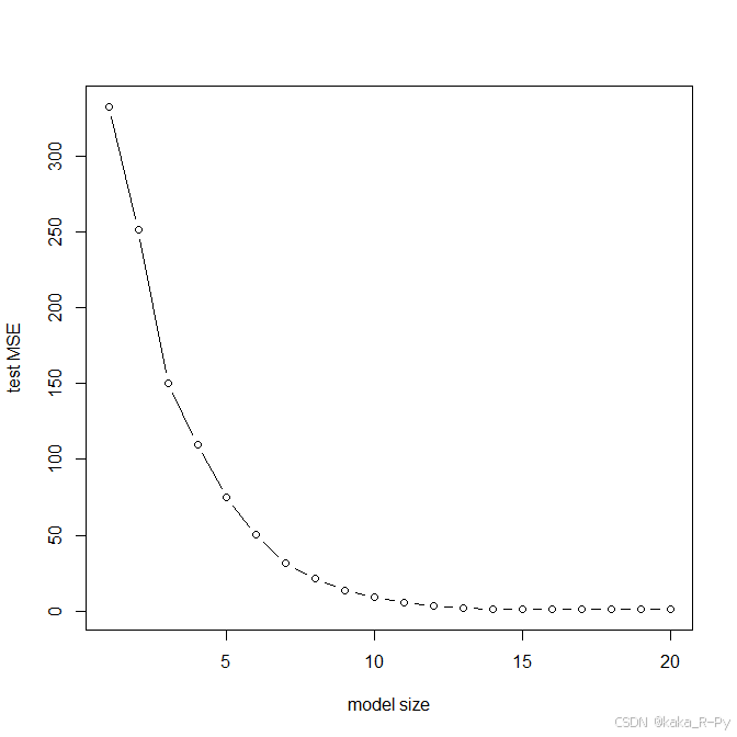
e 当模型含有多少个特征时，测试集MSE最小。

#way1
which.min(val.errors)

16 parameter model has the smallest test MSE.

#way2
which.min(mse1)

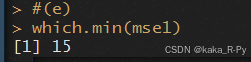
15 parameter model has the smallest test MSE.

f 测试集MSE最小的模型与真实模型比较起来有何不同，比较模型系数。

#way1
coef(regfit.full, id=16)

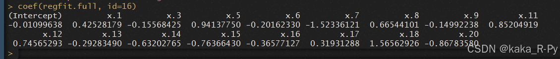
Caught all but one zeroed out coefficient at x.2,x.4,x.10,x.19.

#way2
coefficients(fit1,id=15)

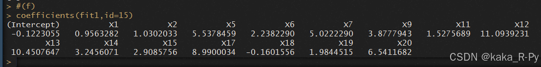
Caught all but one zeroed out coefficient at x.3,x.4,x.8,x.10,x.16.

g 作出$r$在一定范围内取值时$\sqrt{{\sum }_{j=1}^p{\left({\beta }_j-{\hat{\beta }}_j^r\right)}^2}$的图像，其中${\hat{\beta }}_j^r$为包含$r$个预测变量的最优模型中第$j$个系数的估计值。

#way1
val.errors = rep(NA, p)
a = rep(NA, p)
b = rep(NA, p)
for (i in 1:p) {
  coefi = coef(regfit.full, id=i)
  a[i] = length(coefi)-1
  b[i] = sqrt(
    sum((B[x_cols %in% names(coefi)] - coefi[names(coefi) %in% x_cols])^2) +
      sum(B[!(x_cols %in% names(coefi))])^2)
}
plot(x=a, y=b, xlab="number of coefficients",
     ylab="error between estimated and true coefficients")
which.min(b)

Model with 9 coefficients (10 with intercept) minimizes the error between the
estimated and true coefficients. Test error is minimized with 16 parameter model.
A better fit of true coefficients as measured here doesn’t mean the model will have.

#way2
xcol=colnames(x,do.NULL =F,prefix = "X")
s=rep(NA,20)
for(i in 1:20){
  s[i]=sqrt(sum(beta[xcol%in%names(coefficients(fit1,id=i)[-1])]-
                  coefficients(fit1,id=i)[-1])^2+
              sum(beta[!xcol%in%names(coefficients(fit1,id=i)[-1])])^2)
}

plot(1:20,s,type="b",xlab="numbers of coeffieients",
     ylab='error between estimated and true coefficients')
which.min(s)

Model with 15 coefficients (15 with intercept) minimizes the error between the
estimated and true coefficients. Test error is minimized with 15 parameter model.
A better fit of true coefficients as measured here doesn’t mean the model will have.