


二分类 —— 逻辑回归
符号说明
n:输入特征向量的维度
(x,y)(x,y)(x,y) x∈Rnxx \in \mathbb{R}^{n_x}x∈Rnx,y∈{0,1}y \in \{0,1\}y∈{0,1}:一个单独的样本
m:训练集中的训练样本数量,强调是训练集的时候用 mtrainm_{train}mtrain 表示训练样本,用 mtestm_{test}mtest 表示测试样本
{(x(1),y(1)),(x(2),y(2)),…,(x(m),y(m))}\{(x^{(1)},y^{(1)}),(x^{(2)},y^{(2)}),\dots,(x^{(m)},y^{(m)})\}{(x(1),y(1)),(x(2),y(2)),…,(x(m),y(m))}:训练集
训练集:X=[⋮⋮⋮x(1)x(2)⋯x(m)⋮⋮⋮]X = \left[\begin{matrix} \vdots &\vdots & &\vdots\\x^{(1)} &x^{(2)} &\cdots&x^{(m)}\\\vdots &\vdots & &\vdots \end{matrix}\right]X=⎣⎢⎢⎡⋮x(1)⋮⋮x(2)⋮⋯⋮x(m)⋮⎦⎥⎥⎤ X∈Rnx×mX \in \mathbb{R}^{n_x \times m}X∈Rnx×m n行m列
输出:Y=[y(1)y(2)⋯y(m)]Y = \left[\begin{matrix} y^{(1)} &y^{(2)} &\cdots&y^{(m)}\end{matrix}\right]Y=[y(1)y(2)⋯y(m)] Y∈R1×mY \in \mathbb{R}^{1 \times m}Y∈R1×m 1行m列
逻辑回归模型
给定 xxx,x∈Rnxx \in \mathbb{R}^{n_x}x∈Rnx,想到得到 y^\hat yy^,是一个估计的概率:y^=P(y=1∣x)\hat y=P(y=1|x)y^=P(y=1∣x) 0≤y^≤10\leq \hat y \leq 10≤y^≤1 cans
参数:ω∈Rnx\omega \in \mathbb{R}^{n_x}ω∈Rnx,b∈Rb \in \mathbb Rb∈R
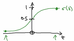
输出:y^=σ(ωTx+b)=σ(z)=11+e−z\hat y =\sigma(\omega^Tx+b) = \sigma(z) = \dfrac{1}{1+e^{-z}}y^=σ(ωTx+b)=σ(z)=1+e−z1 z 正向很大时σ(z)≈1\sigma(z)\approx 1σ(z)≈1,z 负向很大时σ(z)≈0\sigma(z)\approx 0σ(z)≈0,
-
损失函数:衡量单一训练样本的效果
L(y^,y)=−(ylogy^+(1−y)log(1−y^))L(\hat y,y) = - (y\log \hat y+(1-y)\log(1-\hat y))L(y^,y)=−(ylogy^+(1−y)log(1−y^))
if y=1: L(y^,y)=−logy^←L(\hat y,y) = - \log \hat y \leftarrowL(y^,y)=−logy^← want logy^\log\hat ylogy^ large,want y^\hat yy^ large
if y=0: L(y^,y)=−log(1−y^)←L(\hat y,y) = - \log (1-\hat y) \leftarrowL(y^,y)=−log(1−y^)← want log(1−y^\log(1-\hat ylog(1−y^ large,want y^\hat yy^ small -
代价函数:衡量参数w和b在全部训练集上的效果
J(ω,b)=1m∑i=1mL(y^(i),y(i))=−1m∑i=1my(i)logy^(i)+(1−y(i))log(1−y^(i))J(\omega,b) = \frac{1}{m} \sum_{i=1}^m L(\hat y^{(i)},y^{(i)}) =-\frac{1}{m} \sum_{i=1}^m y^{(i)}\log \hat y^{(i)}+(1-y^{(i)})\log(1-\hat y^{(i)})J(ω,b)=m1∑i=1mL(y^(i),y(i))=−m1∑i=1my(i)logy^(i)+(1−y(i))log(1−y^(i))
使用这样的损失函数可以使得代价函数是一个凸函数
梯度下降
Repeat{
ω:=ω−αdJ(ω,b)dw\omega := \omega - \alpha \dfrac{dJ(\omega,b)}{dw}ω:=ω−αdwdJ(ω,b)
b:=b−αdJ(ω,b)dbb := b - \alpha \dfrac{dJ(\omega,b)}{db}b:=b−αdbdJ(ω,b)
}
- α\alphaα 学习率
- 大于1时用偏导,但在编程中都记为 ω:=ω−αdw\omega := \omega - \alpha dwω:=ω−αdw
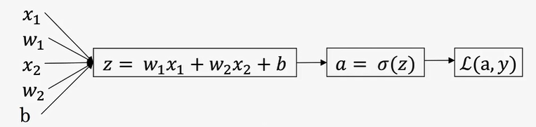
计算图
正向:从左向右计算代价函数,需要优化的函数
反向:从右向左计算导数
逻辑回归的梯度下降
单一样本:真值标签值yyy,两个特征值 x1x_1x1,x2x_2x2,输入参数ω1\omega_1ω1,ω2\omega_2ω2,bbb
正向预测:
z=ωTx+bz = \omega^Tx+bz=ωTx+b
y^=a=σ(z)\hat y = a =\sigma(z)y^=a=σ(z)
L(a,y)=−(yloga+(1−y)log(1−a))L(a,y)=-(y\log a+(1-y)\log(1-a))L(a,y)=−(yloga+(1−y)log(1−a))
反向求导:
da→dL(a,y)da=−ya+1−y1−a\text{da} \rightarrow \dfrac{\mathbb d L(a,y)}{\mathbb da} = -\dfrac{y}{a}+\dfrac{1-y}{1-a}da→dadL(a,y)=−ay+1−a1−y
dz→dL(a,y)dz=dL(a,y)dadadz=a−y←dadz=e−z(1+e−z)2=1(1+e−z)(1−1(1+e−z))=a(1−a)\text{dz}\rightarrow \dfrac{\mathbb d L(a,y)}{\mathbb dz} =\dfrac{\mathbb d L(a,y)}{\mathbb da}\dfrac{\mathbb d a}{\mathbb dz} = a-y \leftarrow \dfrac{\mathbb d a}{\mathbb dz}=\dfrac{e^{-z}}{(1+e^{-z})^2}=\dfrac{1}{(1+e^{-z})}(1-\dfrac{1}{(1+e^{-z})})=a(1-a)dz→dzdL(a,y)=dadL(a,y)dzda=a−y←dzda=(1+e−z)2e−z=(1+e−z)1(1−(1+e−z)1)=a(1−a)
dw1→dL(a,y)dω1=x1dz\text{dw1}\rightarrow \dfrac{\mathbb d L(a,y)}{\mathbb d \omega_1} = x_1\mathbb dzdw1→dω1dL(a,y)=x1dz
dw2→dL(a,y)dω2=x2dz\text{dw2}\rightarrow \dfrac{\mathbb d L(a,y)}{\mathbb d \omega_2} = x_2\mathbb dzdw2→dω2dL(a,y)=x2dz
db→dL(a,y)db=dz\text{db}\rightarrow \dfrac{\mathbb d L(a,y)}{\mathbb d b} = \mathbb dzdb→dbdL(a,y)=dz
m个样本:真值标签值 yyy,两个特征值 x1x_1x1,x2x_2x2,输入参数ω1\omega_1ω1,ω2\omega_2ω2,bbb
~~~~~~~~~~~~~~~~~~~~~~~~~~~~~~~~~~~~~~~~~~~~~~~~~~~~~~~~ J=0,dω1=0,dω2=0,db=0J= 0, \mathbb d\omega_1=0, \mathbb d\omega_2=0,\mathbb db=0J=0,dω1=0,dω2=0,db=0
~~~~~~~~~~~~~~~~~~~~~~~~~~~~~~~~~~~~~~~~~~~~~~~~~~~~~~~~ for i=1 to m:\text{for i=1 to m:}for i=1 to m:
z(i)=ωTx(i)+ba(i)=σ(z)(i)J+=−[y(i)loga(i)+(1−y(i))log(1−a(i))]dz(i)=a(i)−y(i)dω1(i)+=x1(i)dz(i)dω2(i)+=x2(i)dz(i)db+=dz(i)\begin{aligned}
&z^{(i)} = \omega^T x^{(i)}+b\\
&a^{(i)} = \sigma(z)^{(i)}\\
&J +=-[y^{(i)}\log a^{(i)}+(1-y^{(i)})\log(1-a^{(i)})]\\
&\mathbb dz^{(i)} = a^{(i)}-y^{(i)}\\
&\mathbb d\omega_1^{(i)} += x_1^{(i)}dz^{(i)} \\
&\mathbb d\omega_2^{(i)} += x_2^{(i)}dz^{(i)} \\
&\mathbb d b += dz^{(i)}
\end{aligned}z(i)=ωTx(i)+ba(i)=σ(z)(i)J+=−[y(i)loga(i)+(1−y(i))log(1−a(i))]dz(i)=a(i)−y(i)dω1(i)+=x1(i)dz(i)dω2(i)+=x2(i)dz(i)db+=dz(i) ~~~~~~~~~~~~~~~~~~~~~~~~~~~~~~~~~~~~~~~~~~~~~~~~~~~~~~~~ J=J/m,dω1=dω1/m,dω2=dω2/m,db=db/mJ= J/m, \mathbb d\omega_1=\mathbb d\omega_1/m, \mathbb d\omega_2=\mathbb d\omega_2/m, \mathbb db=\mathbb db/mJ=J/m,dω1=dω1/m,dω2=dω2/m,db=db/m
~~~~~~~~~~~~~~~~~~~~~~~~~~~~~~~~~~~~~~~~~~~~~~~~~~~~~~~~ ω1:=ω1−αdω1\omega_1 := \omega_1-\alpha\mathbb d\omega_1ω1:=ω1−αdω1
~~~~~~~~~~~~~~~~~~~~~~~~~~~~~~~~~~~~~~~~~~~~~~~~~~~~~~~~ ω2:=ω2−αdω2\omega_2 := \omega_2-\alpha\mathbb d\omega_2ω2:=ω2−αdω2
~~~~~~~~~~~~~~~~~~~~~~~~~~~~~~~~~~~~~~~~~~~~~~~~~~~~~~~~ b:=b−αdbb := b-\alpha\mathbb dbb:=b−αdb
向量化
X=[⋮⋮⋮x(1)x(2)⋯x(m)⋮⋮⋮]X = \left[\begin{matrix} \vdots &\vdots & &\vdots\\x^{(1)} &x^{(2)} &\cdots&x^{(m)}\\\vdots &\vdots & &\vdots \end{matrix}\right]X=⎣⎢⎢⎡⋮x(1)⋮⋮x(2)⋮⋯⋮x(m)⋮⎦⎥⎥⎤ X∈Rnx×mX \in \mathbb{R}^{n_x \times m}X∈Rnx×m n行m列
Z=[z(1),z(2),⋯ ,z(i)]Z =\left[\begin{matrix}z^{(1)},z^{(2)},\cdots,z^{(i)}\end{matrix}\right]Z=[z(1),z(2),⋯,z(i)]
A=[a(1),a(2),⋯ ,a(i)]=σ(Z)A =\left[\begin{matrix}a^{(1)},a^{(2)},\cdots,a^{(i)}\end{matrix}\right] = \sigma(Z)A=[a(1),a(2),⋯,a(i)]=σ(Z)
~~~~~~~~~~~~~~~~~~~~~~~~~~~~~~~~~~~~~~~~~~~~~~~~~~~~~~~~ for inter in rang(1000):\text{for inter in rang(1000):}for inter in rang(1000):
Z=ωTX+b=np.dot(ω.T,X)+bA=σ(Z)dZ=A−Ydω=1mXdZTdb=1mnp.sum(dZ)ω:=ω−αdωb:=b−αdb
\begin{aligned}
&Z = \omega^TX+b = np.dot(\omega.T,X)+b\\
&A =\sigma(Z)\\
&\mathbb dZ = A -Y\\
&\mathbb d\omega = \dfrac{1}{m}X\mathbb dZ^T\\
&\mathbb db = \dfrac{1}{m}np.sum(\mathbb dZ)\\
&\omega := \omega-\alpha\mathbb d\omega\\
&b := b-\alpha\mathbb db
\end{aligned}
Z=ωTX+b=np.dot(ω.T,X)+bA=σ(Z)dZ=A−Ydω=m1XdZTdb=m1np.sum(dZ)ω:=ω−αdωb:=b−αdb
a logistic regression classifier to recognize cats
import numpy as np
import matplotlib.pyplot as plt
import h5py
import scipy
from PIL import Image
from scipy import ndimage
from lr_utils import load_dataset
%matplotlib inline
def load_dataset():
train_dataset = h5py.File('datasets/train_catvnoncat.h5', "r")
train_set_x_orig = np.array(train_dataset["train_set_x"][:]) # your train set features
train_set_y_orig = np.array(train_dataset["train_set_y"][:]) # your train set labels
test_dataset = h5py.File('datasets/test_catvnoncat.h5', "r")
test_set_x_orig = np.array(test_dataset["test_set_x"][:]) # your test set features
test_set_y_orig = np.array(test_dataset["test_set_y"][:]) # your test set labels
classes = np.array(test_dataset["list_classes"][:]) # the list of classes
train_set_y_orig = train_set_y_orig.reshape((1, train_set_y_orig.shape[0]))
test_set_y_orig = test_set_y_orig.reshape((1, test_set_y_orig.shape[0]))
return train_set_x_orig, train_set_y_orig, test_set_x_orig, test_set_y_orig, classes
# Loading the data (cat/non-cat)
train_set_x_orig, train_set_y, test_set_x_orig, test_set_y, classes = load_dataset()
#Figure out the dimensions and shapes of the problem (m_train, m_test, num_px, ...)
m_train = train_set_x_orig.shape[0]
m_test = test_set_x_orig.shape[0]
num_px = train_set_x_orig.shape[1]
print ("Number of training examples: m_train = " + str(m_train))
print ("Number of testing examples: m_test = " + str(m_test))
print ("Height/Width of each image: num_px = " + str(num_px))
print ("Each image is of size: (" + str(num_px) + ", " + str(num_px) + ", 3)")
print ("train_set_x shape: " + str(train_set_x_orig.shape))
print ("train_set_y shape: " + str(train_set_y.shape))
print ("test_set_x shape: " + str(test_set_x_orig.shape))
print ("test_set_y shape: " + str(test_set_y.shape))
#Reshape the datasets such that each example is now a vector of size (num_px * num_px * 3, 1)
train_set_x_flatten = train_set_x_orig.reshape(train_set_x_orig.shape[0],-1).T
test_set_x_flatten = test_set_x_orig.reshape(test_set_x_orig.shape[0],-1).T
#"Standardize" the data
train_set_x = train_set_x_flatten/255.
test_set_x = test_set_x_flatten/255.
def sigmoid(z):
s = 1/(1+np.exp(-z))
return s
def initialize_with_zeros(dim):
w = np.zeros((dim,1))
b = 0
assert(w.shape == (dim, 1))
assert(isinstance(b, float) or isinstance(b, int))
return w, b
def propagate(w, b, X, Y):
m = X.shape[1]
# FORWARD PROPAGATION (FROM X TO COST)
A = sigmoid(np.dot(w.T,X)+b) # compute activation
cost = -1/m*np.sum(Y*np.log(A)+(1-Y)*np.log(1-A)) # compute cost
# BACKWARD PROPAGATION (TO FIND GRAD)
dw = 1/m*np.dot(X,(A-Y).T)
db = 1/m*np.sum(A-Y)
assert(dw.shape == w.shape)
assert(db.dtype == float)
cost = np.squeeze(cost)
assert(cost.shape == ())
grads = {"dw": dw,
"db": db}
return grads, cost
def optimize(w, b, X, Y, num_iterations, learning_rate, print_cost = False):
costs = []
for i in range(num_iterations):
# Cost and gradient calculation
grads, cost = propagate(w,b,X,Y)
# Retrieve derivatives from grads
dw = grads["dw"]
db = grads["db"]
# update rule
w = w-learning_rate*dw
b = b-learning_rate*db
# Record the costs
if i % 100 == 0:
costs.append(cost)
# Print the cost every 100 training examples
if print_cost and i % 100 == 0:
print ("Cost after iteration %i: %f" %(i, cost))
params = {"w": w,
"b": b}
grads = {"dw": dw,
"db": db}
return params, grads, costs
def predict(w, b, X):
m = X.shape[1]
Y_prediction = np.zeros((1,m))
w = w.reshape(X.shape[0], 1)
# Compute vector "A" predicting the probabilities of a cat being present in the picture
A = sigmoid(np.dot(w.T,X)+b)
for i in range(A.shape[1]):
# Convert probabilities A[0,i] to actual predictions p[0,i]
if A[0,i]<=0.5:
Y_prediction[0,i]=0
else:
Y_prediction[0,i]=1
assert(Y_prediction.shape == (1, m))
return Y_prediction
def model(X_train, Y_train, X_test, Y_test, num_iterations = 2000, learning_rate = 0.5, print_cost = False):
# initialize parameters with zeros
w, b = initialize_with_zeros(X_train.shape[0])
# Gradient descent
parameters, grads, costs = optimize(w, b, X_train, Y_train, num_iterations, learning_rate, print_cost)
# Retrieve parameters w and b from dictionary "parameters"
w = parameters["w"]
b = parameters["b"]
# Predict test/train set examples
Y_prediction_test = predict(w,b,X_test)
Y_prediction_train = predict(w,b,X_train)
# Print train/test Errors
print("train accuracy: {} %".format(100 - np.mean(np.abs(Y_prediction_train - Y_train)) * 100))
print("test accuracy: {} %".format(100 - np.mean(np.abs(Y_prediction_test - Y_test)) * 100))
d = {"costs": costs,
"Y_prediction_test": Y_prediction_test,
"Y_prediction_train" : Y_prediction_train,
"w" : w,
"b" : b,
"learning_rate" : learning_rate,
"num_iterations": num_iterations}
return d
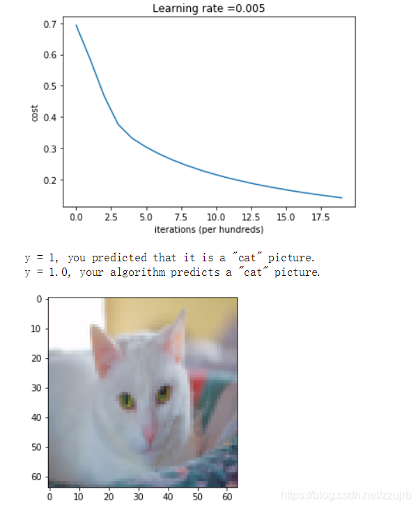
d = model(train_set_x, train_set_y, test_set_x, test_set_y, num_iterations = 2000, learning_rate = 0.005, print_cost = True)
# Plot learning curve (with costs)
plt.figure(1)
costs = np.squeeze(d['costs'])
plt.plot(costs)
plt.ylabel('cost')
plt.xlabel('iterations (per hundreds)')
plt.title("Learning rate =" + str(d["learning_rate"]))
plt.show()
index = 2
plt.figure(2)
plt.imshow(test_set_x[:,index].reshape((num_px, num_px, 3)))
print ("y = " + str(test_set_y[0,index]) + ", you predicted that it is a \"" + classes[int(d["Y_prediction_test"][0,index])].decode("utf-8") + "\" picture.")
# change this to the name of your image file
my_image = "my_image2.jpg"
# We preprocess the image to fit your algorithm.
fname = "images/" + my_image
image = np.array(ndimage.imread(fname, flatten=False))
my_image = scipy.misc.imresize(image, size=(num_px,num_px)).reshape((1, num_px*num_px*3)).T
my_predicted_image = predict(d["w"], d["b"], my_image)
plt.figure(3)
plt.imshow(image)
print("y = " + str(np.squeeze(my_predicted_image)) + ", your algorithm predicts a \"" + classes[int(np.squeeze(my_predicted_image)),].decode("utf-8") + "\" picture.")
Number of training examples: m_train = 209
Number of testing examples: m_test = 50
Height/Width of each image: num_px = 64
Each image is of size: (64, 64, 3)
train_set_x shape: (209, 64, 64, 3)
train_set_y shape: (1, 209)
test_set_x shape: (50, 64, 64, 3)
test_set_y shape: (1, 50)
Cost after iteration 0: 0.693147
Cost after iteration 100: 0.584508
Cost after iteration 200: 0.466949
Cost after iteration 300: 0.376007
Cost after iteration 400: 0.331463
Cost after iteration 500: 0.303273
Cost after iteration 600: 0.279880
Cost after iteration 700: 0.260042
Cost after iteration 800: 0.242941
Cost after iteration 900: 0.228004
Cost after iteration 1000: 0.214820
Cost after iteration 1100: 0.203078
Cost after iteration 1200: 0.192544
Cost after iteration 1300: 0.183033
Cost after iteration 1400: 0.174399
Cost after iteration 1500: 0.166521
Cost after iteration 1600: 0.159305
Cost after iteration 1700: 0.152667
Cost after iteration 1800: 0.146542
Cost after iteration 1900: 0.140872
train accuracy: 99.04306220095694 %
test accuracy: 70.0 %


 773
773

 被折叠的 条评论
为什么被折叠?
被折叠的 条评论
为什么被折叠?
 到【灌水乐园】发言


