


1. 热对流问题的Matlab实现
热对流问题不是本文的重点,对这个问题不了解的话可以参考别的学习资料。OpenMP的基础知识可以参考网上很多资料,也可以参考本博主另外的一片博客《OpenMP基础知识详解及代码示例》。
ly = 51;
aspect_ratio = 2;
lx = aspect_ratio*ly;
delta_x = 1./(ly-2);
Pr = 1.;
Ra = 20000.; % Rayleigh number
gr = 0.001; % Gravity
buoyancy = [0,gr];
Thot = 1; % Heating on bottom wall
Tcold = 0; % Cooling on top wall
T0 = (Thot+Tcold)/2;
delta_t = sqrt(gr*delta_x);
% nu: kinematic viscosity in lattice units
nu = sqrt(Pr/Ra)*delta_t/(delta_x*delta_x);
% k: thermal diffusivity
k = sqrt(1./(Pr*Ra))*delta_t/(delta_x*delta_x);
omegaNS = 1./(3*nu+0.5); % Relaxation parameter for fluid
omegaT = 1./(3.*k+0.5); % Relaxation parameter for temperature
maxT = 80000; % total number of iterations
tPlot = 100; % iterations between successive graphical outputs
tStatistics = 10; % iterations between successive file accesses
% D2Q9 LATTICE CONSTANTS
tNS = [4/9, 1/9,1/9,1/9,1/9, 1/36,1/36,1/36,1/36];
cxNS = [ 0, 1, 0, -1, 0, 1, -1, -1, 1];
cyNS = [ 0, 0, 1, 0, -1, 1, 1, -1, -1];
oppNS = [ 1, 4, 5, 2, 3, 8, 9, 6, 7];
% D2Q5 LATTICE CONSTANTS
tT = [1/3, 1/6, 1/6, 1/6, 1/6];
cxT = [ 0, 1, 0, -1, 0];
cyT = [ 0, 0, 1, 0, -1];
oppT = [ 1, 4, 5, 2, 3];
[y,x] = meshgrid(1:ly,1:lx);
% INITIAL CONDITION FOR FLUID: (rho=1, u=0) ==> fIn(i) = t(i)
fIn = reshape( tNS' * ones(1,lx*ly), 9, lx, ly);
% INITIAL CONDITION FOR TEMPERATURE: (T=0) ==> TIn(i) = t(i)
tIn = reshape( tT' *Tcold *ones(1,lx*ly), 5, lx, ly);
% Except for bottom wall, where T=1
tIn(:,:,ly)=Thot*tT'*ones(1,lx);
% We need a small trigger, to break symmetry
tIn(:,lx/2,ly-1)= tT*(Thot + (Thot/10.));
% Open file for statistics
fid = fopen('thermal_statistics.dat','w');
fprintf(fid,'Thermal Statistics: time-step --- uy[nx/2,ny/2] --- Nu\n\n\n');
% MAIN LOOP (TIME CYCLES)
for cycle = 1:maxT
% MACROSCOPIC VARIABLES
rho = sum(fIn);
T = sum(tIn); %temperature
ux = reshape ( (cxNS * reshape(fIn,9,lx*ly)), 1,lx,ly) ./rho;
uy = reshape ( (cyNS * reshape(fIn,9,lx*ly)), 1,lx,ly) ./rho;
% MACROSCOPIC BOUNDARY CONDITIONS
% NO-SLIP for fluid and CONSTANT at lower and upper
% boundary... periodicity wrt. left-right
% COLLISION STEP FLUID
for i=1:9
cuNS = 3*(cxNS(i)*ux+cyNS(i)*uy);
fEq(i,:,:) = rho .* tNS(i) .* ...
( 1 + cuNS + 1/2*(cuNS.*cuNS) - 3/2*(ux.^2+uy.^2) );
force(i,:,:) = 3.*tNS(i) .*rho .* (T-T0) .* ...
(cxNS(i)*buoyancy(1)+cyNS(i)*buoyancy(2))/(Thot-Tcold);
fOut(i,:,:) = fIn(i,:,:) - omegaNS .* (fIn(i,:,:)-fEq(i,:,:)) + force(i,:,:);
end
% COLLISION STEP TEMPERATURE
for i=1:5
cu = 3*(cxT(i)*ux+cyT(i)*uy);
tEq(i,:,:) = T .* tT(i) .* ( 1 + cu );
tOut(i,:,:) = tIn(i,:,:) - omegaT .* (tIn(i,:,:)-tEq(i,:,:));
end
% MICROSCOPIC BOUNDARY CONDITIONS FOR FLUID
for i=1:9
fOut(i,:,1) = fIn(oppNS(i),:,1);
fOut(i,:,ly) = fIn(oppNS(i),:,ly);
end
% STREAMING STEP FLUID
for i=1:9
fIn(i,:,:) = circshift(fOut(i,:,:), [0,cxNS(i),cyNS(i)]);
end
% STREAMING STEP FLUID
for i=1:5
tIn(i,:,:) = circshift(tOut(i,:,:), [0,cxT(i),cyT(i)]);
end
% MICROSCOPIC BOUNDARY CONDITIONS FOR TEMEPERATURE
%
tIn(5,:,ly) = Tcold-tIn(1,:,ly)-tIn(2,:,ly)-tIn(3,:,ly)-tIn(4,:,ly);
tIn(3,:,1) = Thot-tIn(1,:,1) -tIn(2,:,1) -tIn(4,:,1) -tIn(5,:,1);
% VISUALIZATION
if (mod(cycle,tStatistics)==0)
u = reshape(sqrt(ux.^2+uy.^2),lx,ly);
uy_Nu = reshape(uy,lx,ly); % vertical velocity
T = reshape(T,lx,ly);
Nu = 1. + sum(sum(uy_Nu.*T))/(lx*k*(Thot-Tcold));
fprintf(fid,'%8.0f %12.8f %12.8f\n',cycle,u(int8(lx/2),int8(ly/2))^2, Nu);
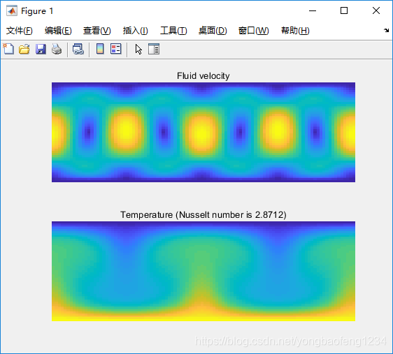
if(mod(cycle,tPlot)==0)
subplot(2,1,1);
imagesc(u(:,ly:-1:1)');
title('Fluid velocity');
axis off; drawnow
subplot(2,1,2);
imagesc(T(:,ly:-1:1)')
title(['Temperature (Nusselt number is ' num2str(Nu) ')']);
axis off; drawnow
end
end
end
fclose(fid);
上述代码我们不做过多的解释,感兴趣的盆友可以参考相关资料学习。
2. 使用OpenMP+Mex+Matlab来实现上述的春Matlab代码
#include <mex.h>
#include <omp.h>
#include <math.h>
#include <string.h>

#define DEBUG 1

// 作元素平移时需要将溢出便捷的索引重新放回到(x,y,z)内
inline int inbound(int idx, int size_t){
	if (idx >= size_t)  return idx - size_t;
	else if (idx < 0)  return idx + size_t;
	else return idx;
}


void mexFunction(int nlhs, mxArray *plhs[], int nrhs, const mxArray *prhs[])
{
	if (nrhs!=2) mexErrMsgTxt("输入参数个数必须为2!\n");
	// 变量定义 ===================================================================
	int  ly = 51, ratio = 2, lx = ratio*ly;
	double dlt_x = 1.0 / (ly - 2), Pr = 1.0, Ra = 20000.0, gr = 0.001, Thot = 1.0, Tcold = 0.0, T0 = (Thot + Tcold) / 2.0;
	double dlt_t = sqrt(gr*dlt_x), nu = sqrt(Pr / Ra)*dlt_t / (dlt_x*dlt_x), k = sqrt(1.0 / (Pr*Ra))*dlt_t / (dlt_x*dlt_x);
	double omegaNS = 1.0 / (3 * nu + 0.5), omegaT = 1.0 / (3 * k + 0.5);
	double buoyancy[2] = { 0, gr };
	int maxT = 80000, tPlot = 100, tStatistics = 10;  // 总迭代次数

	// D2Q9 晶格常数
	double tNS[] = { 4 / 9.0, 1 / 9.0, 1 / 9.0, 1 / 9.0, 1 / 9.0, 1 / 36.0, 1 / 36.0, 1 / 36.0, 1 / 36.0 };
	double cxNS[] = { 0.0, 1.0, 0.0, -1.0, 0.0, 1.0, -1.0, -1.0, 1.0 };
	double cyNS[] = { 0.0, 0.0, 1.0, 0.0, -1.0, 1.0, 1.0, -1.0, -1.0 };
	int oppNS[] = { 1, 4, 5, 2, 3, 8, 9, 6, 7 };

	// D2Q5 晶格常数
	double tT[] = { 1.0 / 3.0, 1.0 / 6.0, 1.0 / 6.0, 1.0 / 6.0, 1.0 / 6.0 };
	double cxT[] = { 0.0, 1.0, 0.0, -1.0, 0.0 };
	double cyT[] = { 0.0, 0.0, 1.0, 0.0, -1.0 };
	double oppT[] = { 1.0, 4.0, 5.0, 2.0, 3.0 };

	int thread_num = omp_get_num_procs();   // 获取CPU总的线程数量

#if DEBUG
	mexPrintf("当前CPU总的线程数量为: %d  \n", thread_num);
#endif
	// 这里获取处理过后的fIn和tIn数据
	double *fIn = (double *)mxGetPr(prhs[0]);  // 9*102*51大小
	double *tIn = (double *)mxGetPr(prhs[1]);  // 5*102*51

	// Size = 1*lx*ly
	double *ux = (double *)malloc(sizeof(double)* 1 * lx*ly);
	double *uy = (double *)malloc(sizeof(double)* 1 * lx*ly);
	double *cuNS = (double *)malloc(sizeof(double)* 1 * lx*ly);
	double *cu = (double *)malloc(sizeof(double)* 1 * lx*ly);

	double *rho = (double *)malloc(sizeof(double)* 1 * lx*ly);
	double *T = (double *)malloc(sizeof(double)* 1 * lx*ly);

	double *fEq = (double *)malloc(sizeof(double)* 9 * lx*ly);
	double *force = (double *)malloc(sizeof(double)* 9 * lx*ly);
	double *fOut = (double *)malloc(sizeof(double)* 9 * lx*ly);

	double *tEq = (double *)malloc(sizeof(double)* 5 * lx*ly);
	double *tOut = (double *)malloc(sizeof(double)* 5 * lx*ly);

#if 1
	mexPrintf("fIn 前20位值: \n");
	for (int i = 0; i < 20; i++)  mexPrintf("%f ", fIn[i]);
	mexPrintf("\n");

	mexPrintf("tIn 前20位值: \n");
	for (int i = 0; i < 20; i++)  mexPrintf("%f ", tIn[i]);
	mexPrintf("\n");
#endif
	// 文件处理这里暂时去除
	for (int i = 1; i <= maxT; i++)   // 最外层循环是时间循环,是不能进行并行的
	{
	    memset(rho, 0, sizeof(double)* 1 * lx*ly); memset(T, 0, sizeof(double)* 1 * lx*ly);
#pragma omp parallel for
		for (int kk = 0; kk < ly; kk++)
		{
			for (int jj = 0; jj < lx; jj++)
			{
				for (int id = 0; id < 9; id++)
				{
					rho[lx*kk+jj] += fIn[9*lx*kk+9*jj+id];
				}

				for (int id = 0; id < 5; id++)
				{
					T[lx*kk + jj] += tIn[5 * lx*kk + 5 * jj + id];
				}
			}
		}

#if 0
		mexPrintf("rho 前20位值: \n");
		for (int ii = 0; ii < 20; ii++)  mexPrintf("%f ", rho[ii]);
		mexPrintf("\n");
		mexPrintf("T 前20位值: \n");
		for (int ii = 0; ii < 20; ii++)  mexPrintf("%f ", T[ii]);
		mexPrintf("\n======================================================================================\n");
		mexPrintf("%f ", T[5048]);
#endif
		//  给ux 和 ux  赋值
		// 每次循环都需要重新初始化ux,uy
		memset(ux, 0, sizeof(double)* 1 * lx*ly); memset(uy, 0, sizeof(double)* 1 * lx*ly);
#pragma omp parallel for
		for (int kk = 0; kk < ly; kk++)	            // 51
		{
			for (int jj = 0; jj < lx; jj++)         // 102
			{
				for (int id = 0; id < 9; id++)      // 求和运算发生在最内层循环,所以不需要归约
				{
					// id 放在内层,是为了让地址连续,以节约运行时间
					ux[kk*lx + jj] += cxNS[id] * fIn[9 * lx*kk + 9 * jj + id] / rho[kk*lx + jj];
					uy[kk*lx + jj] += cyNS[id] * fIn[9 * lx*kk + 9 * jj + id] / rho[kk*lx + jj];
				}
			}
		}

#if 0
		mexPrintf("ux 前20位值: \n");
		for (int ii = 0; ii < 20; ii++)  mexPrintf("%f ", ux[ii]);
		mexPrintf("\n");
		mexPrintf("uy 前20位值: \n");
		for (int ii = 0; ii < 20; ii++)  mexPrintf("%f ", uy[ii]);
		mexPrintf("\n======================================================================================\n");
#endif

		for (int j = 0; j < 9; j++)
		{
#pragma omp parallel for
			for (int k = 0; k < 1 * lx*ly; k++)
			{
				cuNS[k] = 3 * (cxNS[j] * ux[k] + cyNS[j] * uy[k]);
			}

#pragma omp parallel for
			for (int kk = 0; kk < ly; kk++)
			{
				for (int jj = 0; jj < lx; jj++)   // 并行时,可以考虑将内存合并的循环放在外层,以方便每个线程各自访问连续的内存
				{
					fEq[9 * lx*kk + 9 * jj + j] = rho[lx*kk + jj] * tNS[j] * (1 + cuNS[lx*kk + jj] + 0.5*cuNS[lx*kk + jj] * cuNS[lx*kk + jj]
						- 1.5*(ux[lx*kk + jj] * ux[lx*kk + jj] + uy[lx*kk + jj] * uy[lx*kk + jj]));
					force[9 * lx*kk + 9 * jj + j] = 3 * tNS[j] * rho[lx*kk + jj] * (T[lx*kk + jj] - T0)*(cxNS[j] * buoyancy[0] + cyNS[j] * buoyancy[1]) / (Thot - Tcold);
					fOut[9 * lx*kk + 9 * jj + j] = fIn[9 * lx*kk + 9 * jj + j] - omegaNS*(fIn[9 * lx*kk + 9 * jj + j] - fEq[9 * lx*kk + 9 * jj + j]) + force[9 * lx*kk + 9 * jj + j];
				}
			}
		}

#if 0
		mexPrintf("fEq 前20位值: \n");
		for (int ii = 0; ii < 20; ii++)  mexPrintf("%f ", fEq[ii]);
		mexPrintf("\n");
		mexPrintf("force 前20位值: \n");
		for (int ii = 0; ii < 20; ii++)  mexPrintf("%f ", force[ii]);
		mexPrintf("\n");
		mexPrintf("fOut 前20位值: \n");
		for (int ii = 0; ii < 20; ii++)  mexPrintf("%f ", fOut[ii]);
		mexPrintf("\n======================================================================================\n");
#endif


		for (int j = 0; j < 5; j++){
#pragma omp parallel for
			for (int k = 0; k < 1 * lx*ly; k++)
			{
				cu[k] = 3 * (cxT[j] * ux[k] + cyT[j] * uy[k]);
			}

#pragma omp parallel for
			for (int kk = 0; kk < ly; kk++)
			{
				for (int jj = 0; jj < lx; jj++)
				{
					tEq[5 * lx*kk + 5 * jj + j] = T[lx*kk + jj] * tT[j] * (1 + cu[lx*kk + jj]);
					tOut[5 * lx*kk + 5 * jj + j] = tIn[5 * lx*kk + 5 * jj + j] - omegaT*(tIn[5 * lx*kk + 5 * jj + j] - tEq[5 * lx*kk + 5 * jj + j]);
				}
			}
		}

#if 0
		mexPrintf("tEq  后20位值: \n");
		for (int ii = 5 * lx*ly -20 ; ii < 5 * lx*ly; ii++)  mexPrintf("%f ", tEq[ii]);
		mexPrintf("\n");
		mexPrintf("tOut 后20位值: \n");
		for (int ii = 5 * lx*ly - 20; ii < 5 * lx*ly; ii++)  mexPrintf("%f ", tOut[ii]);
		mexPrintf("\n======================================================================================\n");
#endif

		for (int j = 0; j < 9; j++){
#pragma omp parallel for
			for (int jj = 0; jj < lx; jj++)
			{
				fOut[9 * jj + j] = fIn[9 * jj + oppNS[j]-1];
				fOut[9 * lx*(ly - 1) + 9 * jj + j] = fIn[9 * lx*(ly - 1) + 9 * jj + oppNS[j]-1];
			}
		}

#if 0
		mexPrintf("fOut 前20位值: \n");
		for (int ii = 0; ii < 20; ii++)  mexPrintf("%f ", fOut[ii]);
		mexPrintf("\n======================================================================================\n");
#endif

		// 元素平移
#pragma omp parallel for
		for (int kk = 0; kk < ly; kk++)
		{
			for (int jj = 0; jj < lx; jj++)
			{
				for (int j = 0; j < 9; j++)
				{
					fIn[9 * lx*kk + 9 * jj + j] = fOut[9 * lx*inbound((kk - (int)cyNS[j]), ly) + 9 * (inbound(jj - (int)cxNS[j], lx)) + j];
				}
			}
		}

		// 元素平移
#pragma omp parallel for
		for (int kk = 0; kk < ly; kk++)
		{
			for (int jj = 0; jj < lx; jj++)
			{
				for (int j = 0; j < 5; j++){
					tIn[5 * lx*kk + 5 * jj + j] = tOut[5 * lx*inbound((kk - (int)cyNS[j]), ly) + 5 * (inbound(jj - (int)cxNS[j], lx)) + j];
				}
			}
		}
#if 0
		mexPrintf("fIn 前20位值: \n");
		for (int ii = 0; ii < 20; ii++)  mexPrintf("%f ", fIn[ii]);
		mexPrintf("\n\n");
		mexPrintf("tIn 前20位值: \n");
		for (int ii = 0; ii < 20; ii++)  mexPrintf("%f ", tIn[ii]);
		mexPrintf("\n======================================================================================\n");
#endif
#pragma omp parallel for
		for (int j = 0; j < lx; j++){
			tIn[5 * lx*(ly - 1) + 5 * j + 4] = Tcold - tIn[5 * lx*(ly - 1) + 5 * j] - tIn[5 * lx*(ly - 1) + 5 * j + 1] - tIn[5 * lx*(ly - 1) + 5 * j + 2] - tIn[5 * lx*(ly - 1) + 5 * j + 3];
			tIn[5 * j + 2] = Thot - tIn[5 * j] - tIn[5 * j + 1] - tIn[5 * j + 3] - tIn[5 * j + 4];
		}

#if 0
		mexPrintf("tIn 前20位值: \n");
		for (int ii = 0; ii < 20; ii++)  mexPrintf("%f ", tIn[ii]);
		mexPrintf("\n======================================================================================\n");
#endif

		 // 可视化部分放在matlab中去
	}

	// 将结果ux,uy,T输出到 Matlab
	if (nlhs!= 3) mexErrMsgTxt("输出参数个数必须为3!\n");

	plhs[0] = mxCreateDoubleMatrix(lx, ly, mxREAL);  // ux
	plhs[1] = mxCreateDoubleMatrix(lx, ly, mxREAL);  // uy
	plhs[2] = mxCreateDoubleMatrix(lx, ly, mxREAL);  // T

	double *ux_out, *uy_out, *T_out;
	ux_out = mxGetPr(plhs[0]);
	uy_out = mxGetPr(plhs[1]);
	T_out = mxGetPr(plhs[2]);


	memcpy(ux_out,ux,sizeof(double)*lx*ly);
	memcpy(uy_out,uy,sizeof(double)*lx*ly);
	memcpy(T_out,T,sizeof(double)*lx*ly);

	free(ux);free(uy);free(cuNS);free(cu);free(rho);free(T);
	free(fEq);free(force);free(fOut);free(tEq);free(tOut);
}
上述代码的基本流程是:
1.  利用mex接口从matlab空间中获取数据;

2.  在C++空间中创建变量、分配地址;

3.  并行实现算法

4.  将结果输出给matlab;
3. Matlab中编译并运行OpenMP C++ 代码
clear;
clc;
ly           = 51;
aspect_ratio = 2;
lx           = aspect_ratio*ly;
delta_x      = 1./(ly-2);
Pr           = 1.;
Ra           = 20000.; % Rayleigh number
gr           = 0.001;  % Gravity
buoyancy     = [0,gr];

Thot  = 1; % Heating on bottom wall
Tcold = 0; % Cooling on top wall
T0 = (Thot+Tcold)/2;

delta_t = sqrt(gr*delta_x);
% nu: kinematic viscosity in lattice units
nu      = sqrt(Pr/Ra)*delta_t/(delta_x*delta_x);
% k: thermal diffusivity
k       = sqrt(1./(Pr*Ra))*delta_t/(delta_x*delta_x);
omegaNS = 1./(3*nu+0.5); % Relaxation parameter for fluid
omegaT  = 1./(3.*k+0.5); % Relaxation parameter for temperature

maxT   = 80000;    % total number of iterations
tPlot  = 100;      % iterations between successive graphical outputs
tStatistics = 10;  % iterations between successive file accesses

% D2Q9 LATTICE CONSTANTS
tNS   = [4/9, 1/9,1/9,1/9,1/9, 1/36,1/36,1/36,1/36];
cxNS  = [  0,   1,  0, -1,  0,    1,  -1,  -1,   1];
cyNS  = [  0,   0,  1,  0, -1,    1,   1,  -1,  -1];
oppNS = [  1,   4,  5,  2,  3,    8,   9,   6,   7];

% D2Q5 LATTICE CONSTANTS
tT   = [1/3, 1/6, 1/6, 1/6, 1/6];
cxT  = [  0,   1,   0,  -1,   0];
cyT  = [  0,   0,   1,   0,  -1];
oppT = [  1,   4,   5,   2,   3];

[y,x] = meshgrid(1:ly,1:lx);

% INITIAL CONDITION FOR FLUID: (rho=1, u=0) ==> fIn(i) = t(i)
fIn = reshape( tNS' * ones(1,lx*ly), 9, lx, ly);

% INITIAL CONDITION FOR TEMPERATURE: (T=0) ==> TIn(i) = t(i)
tIn = reshape( tT' *Tcold *ones(1,lx*ly), 5, lx, ly);
% Except for bottom wall, where T=1
tIn(:,:,ly)=Thot*tT'*ones(1,lx);
% We need a small trigger, to break symmetry
tIn(:,lx/2,ly-1)= tT*(Thot + (Thot/10.));

a=input('请选择串行还是并行执行程序(0 并行/ 1 串行):');

if a==0
    % 编译cpp代码,加入并行选项
    mex HeatConvectionP.cpp   OPTIMFLAGS="-O2 -DNDEBUG /openmp"
elseif a==1
    % 编译cpp串行代码
    mex HeatConvectionS.cpp
end

% 运行代码
tic;[ux,uy,T]=HeatConvectionS(fIn,tIn);toc

% 绘图
u     = sqrt(ux.^2+uy.^2);
Nu    = 1. + sum(sum(uy.*T))/(lx*k*(Thot-Tcold));

subplot(2,1,1);
imagesc(u(:,ly:-1:1)');
title('Fluid velocity');
axis off; drawnow
subplot(2,1,2);
imagesc(T(:,ly:-1:1)')
title(['Temperature (Nusselt number is ' num2str(Nu) ')']);
axis off; drawnow
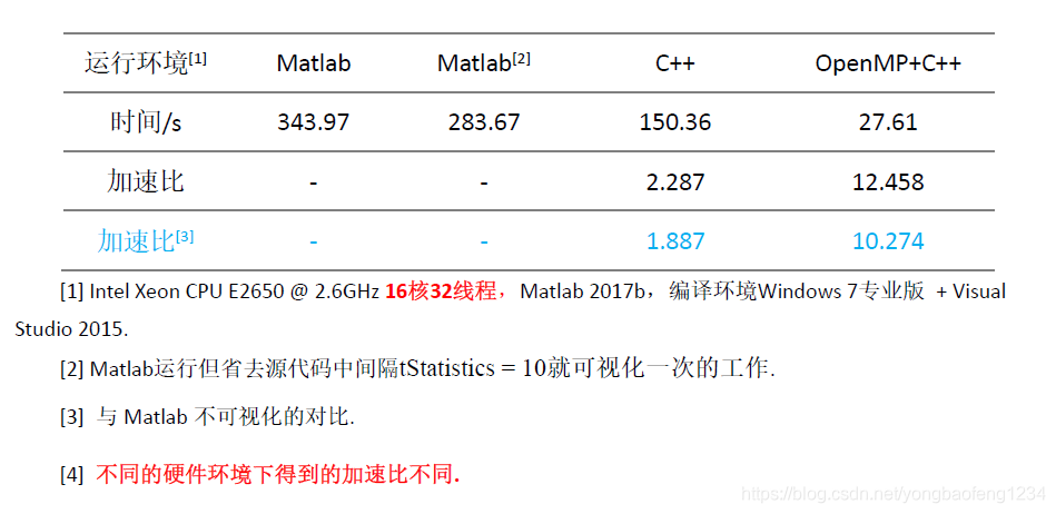
4. 运行结果和并行效率对比
加速效率对比:
5. 程序说明
5.1 Mex接口
本文没有采用纯C++或者Fortran编码方式,而是采用了Matlab + CPP + OpenMP混合编程的方式, 主要出于两个方面的考虑:
1)C++/Fortran的数值处理方便程度远逊色于Matlab,比如代码里的reshape等函数,在C++/Fortran里实现都需要很多的代码,而数据的预处理并不是本文的重点,本文的重点在于加快核心程序的执行速度,并行数据预处理的时间本身也不长 ;
2)mex接口使得在matlab直接调用C++/Fortran成为可能,前者为后两者提供了丰富的API,这样不仅方便与C++/Fortran之间的数据交互,而且很容易将C++/Fortrande运行结果使用Matlab进行可视化出来,而不是在C++中运行完程序将数据保存成文件,又重写编写Matlab程序读取数据文件进行可视化或者后处理 ;
5.2 可视化
虽然本程序在Matlab中运行会花费较长时间,但是除以迭代次数Tmax=80000,其实每个迭代步的花费时间并不长,具体为没步骤s左右。这种情况下。如果每步骤都进行图像可视化是非常耗费时间的,所以表中分别对每步都可视化和不可视化(或者说只进行最后一步可视化)分别进行了计时,可以看到每步都可视化的程序耗时要多出很多。出于此考虑,OpenMP的实现在调试正确后,中间过程也不进行可视化以节约时间,而且混合编程的可视化需要将数据在C++和Matlab之间传递,这又会增加程序的耗时。在实际应用中,如果真的需要,我们可以考虑在OpenMP执行一定的步数后(如500步)可视化一次,毕竟一次可视化的数据拷贝时间和500迭代的计算时间相比,是可以忽略不计的。
5.3 并行优化
OpenMP代码实现的时候,考虑到C++存储矩阵的顺序是按行存储的,而Matlab是按列存储的,所以为了在并行时尽量合并内存的访问,我们尽可能将内存连续的循环放在最内侧,尽可能让缓存命中的几率更大,以提高程序的执行效率。


 1972
1972

 被折叠的 条评论
为什么被折叠?
被折叠的 条评论
为什么被折叠?
 到【灌水乐园】发言


