Build in the Cloud: How the Build System works

This is the second in a four part series describing how we use the cloud to scale building and testing of software at Google. This series elaborates on a presentation given during the Pre-GTAC 2010 event in Hyderabad. Please see our first post in the series for a description how we access our code repository in a scalable way. To get a sense of the scale and details on the types of problems we are solving in Engineering Tools at Google take a look at this post.

As you have learned in the previous post, at Google every product is constantly building from head. In this article we will go into a little more detail in how we tell the build system about the source code and its dependencies. In a later article we will explain how we take advantage of having this exact knowledge to distribute the builds at Google across a large cluster of machines and share build results between developers.

From some of the feedback we got for our first posts it is clear that you want to see how we actually go about describing the dependencies we use to drive our build and test support.

At Google we partition our source code into smaller entities that we call packages. You can think of a package as a directory containing a number of source files and a description of how these source files should get translated into build outputs. The files describing that are all called BUILD and the existence of a BUILD file in a directory makes that directory into a package.

All packages reside in a single file tree and the relative path from the root of that tree to the directory containing the BUILD file is used as a globally unique identifier for the package. This means that there is a 1:1 relationship between package names and directory names.

Within a BUILD file we have a number of named rules describing the build outputs of the package. The combination of package name and rule name uniquely identifies the rule. We call this combination a label and we use labels to describe dependencies across rules.

Let’s look at an example to make this a little more concrete:

/search/BUILD:
cc_binary(name = ‘google_search_page’,
deps = [ ‘:search’,
‘:show_results’])

cc_library(name = ‘search’,
srcs = [ ‘search.h’,‘search.cc’],
deps = [‘//index:query’])

/index/BUILD:

cc_library(name = ‘query’,
srcs = [ ‘query.h’, ‘query.cc’, ‘query_util.cc’],
deps = [‘:ranking’,
‘:index’])

cc_library(name = ‘ranking’,
srcs = [‘ranking.h’, ‘ranking.cc’],
deps = [‘:index’,
‘//storage/database:query’])

cc_library(name = ‘index’,
srcs = [‘index.h’, ‘index.cc’],
deps = [‘//storage/database:query’])

This example shows two BUILD files. The first one describes a binary and a library in the package //search and the second one describes several libraries in the package //index. All rules are named using the name attribute, You can see the dependencies expressed in the deps attribute of each rule. The ‘:’ separates the package name from the name of the rule. Dependencies on rules in a different package start with a “//” and dependencies on rules in the same package can just omit the package name itself and start with a ‘:’. You can clearly see the dependencies between the rules. If you look carefully you will notice that several rules depend on the same rule //storage/database:query, which means that the dependencies form a directed graph. We require that the graph is acyclic, so that we can create an order in which to build the individual targets.

 

Here is a graphical representation of the dependencies described above:

 

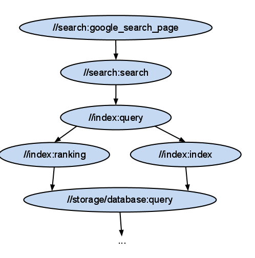
You can also see that instead of referring to concrete build outputs as typically happens in make based build systems, we refer to abstract entities. In fact a rule like cc_library does not necessarily produce any output at all. It is simply a way to logically organize your source files. This has an important advantage that our build system uses to make the build faster. Even though there are dependencies between the different cc_library rules, we have the freedom to compile all of the source files in arbitrary order. All we need to compile ‘query.cc’ and ‘query_util.cc’ are the header files of the dependencies ‘ranking.h’ and ‘index.h’. In practice we will compile all these source files at the same time, which is always possible unless there is a dependency on an actual output file of another rule.

In order to actually perform the build steps necessary we decompose each rule into one or more discrete steps called actions. You can think of an action as a command line and a list of the input and output files. Output files of one action can be the input files to another action. That way all the actions in a build form a bipartite graph consisting of actions and files. All we have to do to build our target is to walk this graph from the leaves - the source files that do not have an action that produces them - to the root and executing all the actions in that order. This will guarantee that we will always have all the input files to an action in place prior to executing that action.

 

An example of the bipartite action graph for a small number of targets. Actions are shown in green and files in yellow color:

 

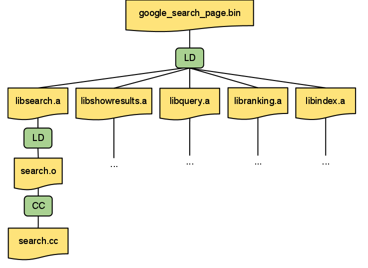
We also make sure that the command-line arguments of every action only contain file names using relative paths - using the relative path from the root of our directory hierarchy for source files. This and the fact that we know all input and output files for an action allows us to easily execute any action remotely: we just copy all of the input files to the remote machine, execute the command on that machine and copy the output files back to the user’s machine. We will talk about some of the ways we make remote builds more efficient in a later post.

All of this is not much different from what happens in make. The important difference lies in the fact that we don’t specify the dependencies between rules in terms of files, which gives the build system a much larger degree of freedom to choose the order in which to execute the actions. The more parallelism we have in a build (i.e. the wider the action graph) the faster we can deliver the end results to the user. At Google we usually build our solutions in a way that can scale simply by adding more machines. If we have a sufficiently large number of machines in our datacenter, the time it takes to perform a build should be dominated only by the height of the action graph.

What I describe above is how a clean build works at Google. In practice most builds during development will be incremental. This means that a developer will make changes to a small number of source files in between builds. Building the whole action graph would be wasteful in this case, so we will skip executing an action unless one or more of its input files change compared to the previous build. In order to do that we keep track of the content digest of each input file whenever we execute an action. As we mentioned in the previous blog post, we keep track of the content digest of source files and we use the same content digest to track changes to files. The FUSE filesystem described in the previous post exposes the digest of each file as an extended attribute. This makes determining the digest of a file very cheap for the build system and allows us to skip executing actions if none of the input files have changed.

Stay tuned! In this post we explained how the build system works and some of the important concepts that allow us to make the build faster. Part three in this series describes how we made remote execution really efficient and how it can be used to improve build times even more!

- Christian Kemper