原文:https://seblagarde.wordpress.com/2011/08/17/hello-world/
With permission of my company : Dontnod entertainment http://www.dont-nod.com/
This last year sees a growing interest for physically based rendering. Physically based shading simplify parameters control for artists, allow more consistent look under different lighting condition and have better realistic look. As many game developers, I decided to introduce physical based shading model to my company. I started this blog to share what we learn. The blog post is divided in two-part.
I will first present the physical shading model we chose and what we add in our engine to support it : This is the subject of this post. Then I will describe the process of making good data to feed this lighting model: Feeding a physically based shading model . I hope you will enjoy it and will share your own way of working with physically based shading model. Feedback are welcomed!
Notation of this post can be found in siggraph 2010 Physically-Based Shading Models in Film and Game Production Naty Hoffman’s paper [2].
Working with a physically based shading model imply some changes in a game engine to fully support it. I will expose here the physically based rendering (PBR) way we chosed for our game engine.
When talking about PBR, we talk about BRDF, Fresnel, energy conserving, Microfacet theory, punctual light sources equation… All these concepts are very well described in [2] and will not be reexplained here.
Our main lighting model is composed of two-part: Ambient lighting and direct lighting. But before digging into these subjects, I will talk about some magic numbers.
Normalization factor
I would like to clarify the constant we find in various lighting model. The energy conservation constraint (the outgoing energy cannot be greater than the incoming energy) requires the BRDF to be normalized. There are two different approaches to normalize a BRDF.
Normalize the entire BRDF
Normalizing a BRDF means that the directional-hemispherical reflectance (the reflectance of a surface under direct illumination) must always be between 0 and 1 : . This is an integral over the hemisphere. In game
![]() corresponds to the diffuse color
corresponds to the diffuse color ![]() .
.
For lambertian BRDF, ![]() is constant. It mean that
is constant. It mean that and we can write
![]()
As a result, the normalization factor of a lambertian BRDF is ![]()
For original Phong (the Phong model most game programmer use) normalization factor is
![]()
For Phong BRDF (just mul Phong by ![]() See [1][8])
See [1][8]) normalization factor becomes
![]()
For Binn-Phong normalization factor is
![]()
For Binn-Phong BRDF normalization factor is
![]()
Derivation of these constants can be found in [3] and [13]. Another good sum up is provide in [27].
Note that for Blinn-Phong BRDF, a cheap approximation is given in [1] as : ![]()
There is a discussion about this constant in [4] and here is the interesting comment from Naty Hoffmann
About the approximation we chose, we were not trying to be strictly conservative (that is important for multi-bounce GI solutions to converge, but not for rasterization).
We were trying to choose a cheap approximation which is close to 1, and we thought it more important to be close for low specular powers.
Low specular powers have highlights that cover a lot of pixels and are unlikely to be saturating past 1.
When working with microfacet BRDFs, normalize only microfacet normal distribution function (NDF)
A Microfacet distribution requires that the (signed) projected area of the microsurface is the same as the projected area of the macrosurface for any direction v [6]. In the special case v = n:
The integral is over the sphere and cosine factor is not clamped.
For Phong distribution (or Blinn distribution, two name, same distribution) the NDF normalization constant is ![]()
Derivation can be found in [7]
Direct Lighting
Our direct lighting model is composed of two-parts : direct diffuse + direct specular
Direct diffuse is the usual Lambertian BRDF : ![]()
Direct specular is the microfacet BRDF describe by Naty Hoffman in [2] :
Naty used the Microfacet BRDF definition found in [6] :
The constant ![]() comes from the normalized Blinn NDF constant
comes from the normalized Blinn NDF constant ![]() divided by 4 (the factor included in microfacet BRDF).
divided by 4 (the factor included in microfacet BRDF).
In game we use punctual light sources (directional/point/spot lights…) for direct lighting. The lighting unit for these light sources is specified as the color a white lambertian surface would have when illuminated by the light from a direction parallel to the surface normal. The punctual light equation is defined by :
See derivation in [2].
Applying our lighting model to the punctual light equation :
So, in our game lighting formula is :
Our specular shader code is:
float3 FresnelSchlick(float3 SpecularColor,float3 E,float3 H)
{
    return SpecularColor + (1.0f - SpecularColor) * pow(1.0f - saturate(dot(E, H)), 5);
}
FresnelSchlick(SpecularColor, L, H) * ((SpecularPower + 2) / 8 ) * pow(saturate(dot(N, H)), SpecularPower) * dotNL;
Remark: For the normalized Phong model mostly use in game engine, we should use:
The ![]() term has disappeard from the normalization constant.
term has disappeard from the normalization constant.
Added note:
Energy conservation should take into account the diffuse and specular term together. For simple no-physical based model (model without Fresnel like Phong or Blinn-Phong), respecting the constraint is sufficient. It can be achieved with
![]()
For a more PBR compliant model such as ours this is more difficult because we must take into account the Fresnel term. Just using “1 – Fresnel” is not valid. See [1] or [10] for details. We aren’t handling this in our game.
implementation detail
Specular Power ![]()
Real world SpecularPower values range from 0.1 to more than 100000 [15]. It is very difficult for game engines to deal with such a range without storing SpecularPower on 16bits instead of the usual 8bits. Obviously, we didn’t do this and try to use the 8bits available as best as possible.
Most game engines store SpecularPower in the 0-255 range fitting nicely an 8bit texture. Which is rather a bad way for PBR. As in [2] we used a gloss factor ![]() defined in the 0(rough)-1(smooth) range and stored in 8bit.
defined in the 0(rough)-1(smooth) range and stored in 8bit.
The decoding follow this equation ![]() which allows a perceptual linear distribution.
which allows a perceptual linear distribution.
SpecularPower = exp2(10 * gloss + 1)
Remark.With very smooth surfaces (with high SpecularPower values) like water, we can get really strong highlight. Using half in shader instead of float for specular lighting resulted in banding artifacts. So some parts of our specular calculation are using float.
Specular
In game we deals with two category of material: dielectric and metal material.
Dielectric material (water, glass, skin, wood, hair, leather, plastic, stone, concrete…) have white specular reflectance. Metals have spectral (mean use RGB color) specular reflectance. But some metals have same Fresnel behavior at all wavelength (like aluminium). See [1] or [2].
With this in mind, it can be tempting for performance to have a separated shader for non-spectral (the most common material) and spectral specular material. This could reduce storage (require 1 channel in texture instead of 3) and save few mul/mad instruction in shader (the pow is not affected).
However, a common trick to save drawcall is to merge material ID (3DS Max definition) together to have only one drawcall per object. Dieletric and metal material on an object now shared the same texture and the same shader. To deal with this advantage, we only have one spectral specular lighting shader. The instruction penalty is really low and texture storage is not a big deal either as specular tend to be constant and require low resolution texture.
I must add that we have a forward engine. Deferred engine with only one channel for specular color will not deal with spectral specular.
Added note:
Gotanda in [13] used a dedicated metal lighting shader. This metal lighting model is based on [14] which details an “Error compensation” that creates the particular curve around Brewster’s angle with metals. According to Gotanda, this only creates a subtle difference [19]. We didn’t consider it for our game.
Optimization
Edit : This section is not up to date. Read Spherical Gaussian approximation for Blinn-Phong, Phong and Fresnel for full details.
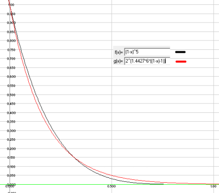
FresnelSchlick in the specular lighting equation can be optimized. Optimization is often performed by using a factor of 4 instead of 5 to generate better instructions/scheduling. It is possible to get better performance without sacrifying the factor 5 by switching the pow in FresnelSchlick to a spherical gaussian (SG) approximation [16][17][18] defined as:
SphericalGaussian(A,B, p) = exp((p+1) * (dot(A,B) – 1)) credit to Matthew Jones :
float SphericalGaussianApprox(float CosX, float ModifiedSpecularPower)
{
    return exp2(ModifiedSpecularPower * CosX - ModifiedSpecularPower);
}
#define OneOnLN2_x6 8.656170 // == 1/ln(2) * 6   (6 is SpecularPower of 5 + 1)
float3 FresnelSchlick(float3 SpecularColor,float3 E,float3 H)
{
    // In this case SphericalGaussianApprox(1.0f - saturate(dot(E, H)), OneOnLN2_x6) is equal to exp2(-OneOnLN2_x6 * x)
    return SpecularColor + (1.0f - SpecularColor) * exp2(-OneOnLN2_x6 * saturate(dot(E, H)));
}
Following figure compare FresnelSchlick SG approximation to FresnelSchlick
We apply a similar optimization for Blinn distribution as in [17].
The deal is just to see that for low specular power exp((p+1) * (dot(A,B) – 1)) fit nicely and for high specular power we can drop the +1. This is what [17] do without mentionning it. Low specular value will be wrong but nobody will notice it.
Added note:
Instead of using p+1 in the fresnel approximation, you can tweak the added value between 0-1 depends on what best fit what you want for your given specular power [18].
Ambient Lighting
Ambient lighting is compose of two-part : Ambient diffuse + Ambient specular
Ambient diffuse
Ambient diffuse is based on static global illuminated lightmap (containing only indirect lighting) for environment and SH irradiance volume for dynamic object. PBR is really important for global illumination solver to avoid creating lighting with multiple bounce. I will not talk about ambient diffuse. There is several good reference on it.
Ambient specular
For ambient specular we take the now common solution to apply prefiltered environment map (cube map) on everything, even “matte” object. This make sense because in real world, every object have some specular lighting [9]. And this help to deal with metal material which should have no diffuse component. Care must be taken to ensure that highlight blurring (specular lighting coming from punctual light sources which are not present in the cubemap) is consistent with cubemap blurring (specular coming from cubemap) [20]. Most game use an eye calibrated prefiltered cubemap. A method of eye calibration is describe in [2].
We tried to be more “correct” for our game.
Prefiltered cubemap
A cubemap contain incoming lighting. Goal is to prefilter cubemap to store reflected light:
The large number of input (view direction, Fresnel etc…) imply large storage that we can’t afford. We instead approximate ambient specular by convolving the cubemap with a Phong lobe in the spirit of [11]:
and apply the Fresnel term at runtime.
This mean that our ambient specular will not match our Blinn-Phong highlight. But with a single environment lookup, we are only able to match Phong highlight.
AMD Cubemapgen tool (which deal with proper filtering and edge fixup) [11] is generally used to prefilter cubemap, but it don’t offer a cosines power weighting filter. HDRShop [21] can perform this kind of filtering but require a conversion to latlong environment format. We write our custom version inside our engine (Edit: The source code of AMD Cubemapgen are now available and can be found at [11]. It is easy to add a cosines power weighting filter. The source has been uploaded to a google code project [26] and are subject to evolve).
When using prefiltered cubemap at runtime, goal is to select a correct mip level based on ![]() . For performance reason, we use a simple linear function: (1-s) * “number of mipmap of cubemap” with gloss parameter (s) in the range 0-1. This linear function must be take in count when generating prefiltered cubemap. At mip level generation, we recover the SpecularPower based on the number of mipmap then use it to prefilter current mip level. :
. For performance reason, we use a simple linear function: (1-s) * “number of mipmap of cubemap” with gloss parameter (s) in the range 0-1. This linear function must be take in count when generating prefiltered cubemap. At mip level generation, we recover the SpecularPower based on the number of mipmap then use it to prefilter current mip level. :
for (INT MipIndex = 0; MipIndex < NumMipmap; MipIndex++)
{
    float gloss = 1.0 - MipIndex / (NumMipmap - 1)
    // Use same formula than in the shader code
    int SpecularPower = round(pow(2, 10 * gloss + 1));
    PrecomputeEnvMap(MipIndex,SpecularPower)
}
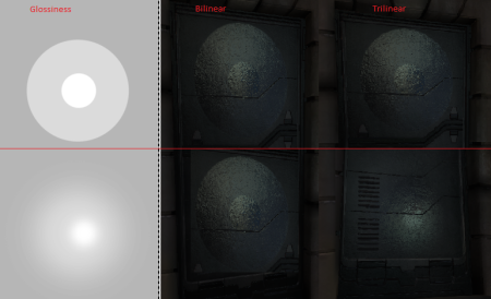
In shader, to recover in between blurriness, we set trilinear interpolation with clamp texture address mode for the prefiltered cubemap . With this method, we handle different cubemap resolutions without the need to eye recalibrate highlight matching.
Here is an in-engine screenshot (click for full res):
From Left to Right there is 11 spheres using our specular model. Each have a different SpecularPower (2048-1024-512-256-128-64-32-16-8-4-2). All spheres display a prefiltered cubemap and a highlight from a directional light (the white point) and no bloom postprocess is present.
On the top row, as a reference, spheres use 128x128x6 prefiltered cubemap at full resolution (so no mipmap chain). On the bottom row, spheres use 128x128x6 prefiltered cubemap with mipmap chain generated with the detailed method. See how the highlight blurring is consistent with the cubemap blurring and how the mipmap chain approximation is close to the reference solution for SpecularPower > 32. Below the resolution of mipmap start to be a problem but result quality is sufficient for us.
In practice:
– We used HDR cubemap of 128x128x6 with mip level going until 4×4 (Remember that our blurring is based on number of mipmap) compress and convert to sRGB similar to [2] then transformed in DXT1.
– As we use cosines power prefiltering, even a SpecularPower of 2048 still blur the cubemap. Perfect cubemap can be get only with a SpecularPower > 16000. To solve this, we add an option for artists to “bias” the specular power range when generating prefiltered cubemap and apply a SpecularPower remapping to still consistent.
– If you tell me “Is this work really required ?”, I will say “probably not”. You can get good result with standard eye matching. Flexibility in cubemap size still a good point and if you can afford 16bit SpecularPower and higher cubemap resolution, it could be a good solution.
– The prefiltered cubemap must be trilinear filtered, as show in picture (click for full rez):
Ambient specular formula
As describe above our ambient specular is composed of a Fresnel term apply at runtime and a cosines power term (Phong lobe) baked in a prefiltered cubemap. We apply the Fresnel term with normal and view vector as in [2]:
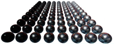
Here is a screenshot (click for full res):
Each sphere is parameterized with our specular model (ambient specular + direct specular). Non spectral (grey) specular value increase from left (0) to right (1). Gloss value increase from top (0 – rough) to bottom (1 – smooth).
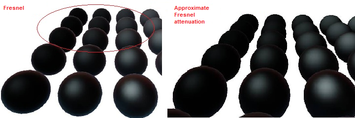
Applying Fresnel term to prefiltered cubemap has a bad effect of always showing high specular color at edge, even for rough surface.
The same Fresnel term which is appropriate for unfiltered environment maps (i.e. perfectly smooth mirror surfaces) is not appropriate for filtered environment maps since there you are averaging incoming light colors from many directions, but using a single Fresnel value computed for the reflection direction. The correct function has similar values as the regular Fresnel expression at v=n, but at glancing angle it behaves differently. In particular, the lerp(from base specular to white) does not go all the way to white at glancing angles in the case of rough surfaces [22].
We approximate this “fresnel attenuation” empirically by introducing a fudge factor (taking count of gloss) in Fresnel equation to get pleasant visual result:
Here is the shader code of our ambient specular:
float3 FresnelSchlickWithRoughness(float3 SpecularColor,float3 E,float3 N,float Gloss)
{
    return SpecularColor + (max(Gloss, SpecularColor) - SpecularColor) * pow(1 - saturate(dot(E, N)), 5);
}
float3 SpecularEnvmap(float3 E,float3 N,float3 R,float3 SpecularColor, float Gloss)
{
    float3 Envcolor = texCUBElod(EnvironmentTexture, float4(R, EnvMapMipmapScaleBias.x * Gloss + EnvMapMipmapScaleBias.y)).rgb;
    return FresnelSchlickWithRoughness(SpecularColor, N, E, Gloss) * Envcolor.rgb * EnvMapScaleAndModulate; // EnvMapScaleAndModulate is used to decompress range
}
(Click for full res)
Illustration of the above formula. Top-Left zoom of the last spheres screenshot. Spheres have low specular and low gloss value. See how the fresnel effect is visible on the left image and have annoying edge highlight.
Added note:
Lazarov in [25] handle the Fresnel attenuation with a modified Fresnel equation : .
According to the slide comment, his factor needs more tuning and the current approximation is a bit too bright, especially for rough surfaces. Caution, the equation is done to match the Fresnel and visibility term used by Dimitar Lazarov, if you don’t use the same visibility term, you must find a new equation.
Another approach to handle this fresnel behavior is describe in [13]. The paper define a custom ambient BRDF with one part of the specular BRDF baked into a volume texture and the other part in the prefiltered cubemap.
texCubeLod can cause texture trashing with smooth surface (high gloss value). [23] Describe a way to minimize this by sampling two times the cubemap. We don’t do this. However, on one particular platform we are able to get
hardware selected mip. The mip use will be max of hardware selected mip and gloss selected mip.
Another way to reduce texture trashing is to apply a gloss texture filtering as describe in [24] or [25]





 本文介绍了一种物理渲染模型的实现细节,包括模型的选择、游戏引擎中的实现方式、直接光照和环境光照的处理方法等。文章还探讨了如何优化计算过程以提高效率。



 1535
1535

 被折叠的 条评论
为什么被折叠?


