


用python构建一个简单的ANN(也称NN)网络
此代码实现了一个简单的神经网络训练过程
通过自定义的前向传播和反向传播过程,对输入数据进行训练。网络采用了两层全连接隐藏层,解构参考下图,每层都有可选择的激活函数(Sigmoid或ReLU)。
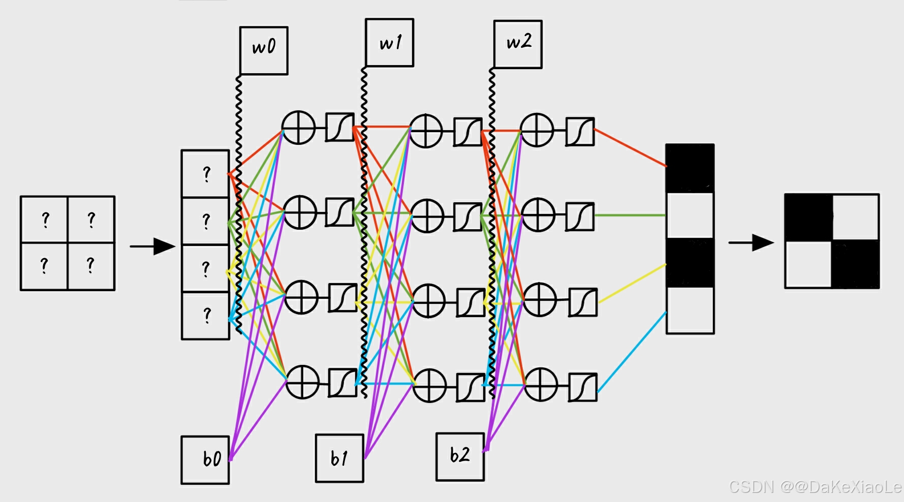
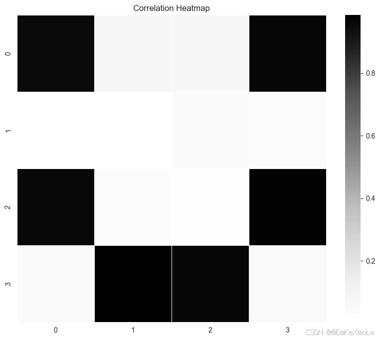
最终实现由随机产生的4x4的随机矩阵,
通过神经网络,生成我们初始规定的4x4图像数据,作为target图像。如下图

核心功能包括:
- 热力图可视化:通过 matplotlib 和 seaborn 绘制数据的热力图。
- 神经网络前向传播:计算网络每层的输出结果。
- 反向传播:计算各层的梯度,并根据损失函数更新权重和偏置。
- 损失计算:使用均方误差(MSE)作为损失函数,并在每次迭代后计算新的损失值。
- 可视化输出结果:使用 TensorBoard 保存并展示训练过程中的输出图像。
代码说明
相应库文件
import matplotlib.pyplot as plt
import seaborn as sns
import numpy as np
import io  # 用于在内存中保存图像
from PIL import Image  # 用于打开并转换图像
from torch.utils.tensorboard import SummaryWriter
定义目标target图像及网络参数
# 显示初始图像,生成一个简单的4x4图像数据作为target图像
img = np.array([[1, 0, 0, 1],
                [0, 0, 0, 0],
                [1, 0, 0, 1],
                [0, 1, 1, 0]])
show_pic(img)  # 可视化该图像
writer = SummaryWriter('logs')  # TensorBoard日志记录器

# 定义每层神经元数量
num_hidden_layer0 = 16  # 第一隐藏层的神经元数量
num_hidden_layer1 = 16  # 第二隐藏层的神经元数量

# 定义学习率
learning_rate = 0.5

# 定义循环训练次数
times = 500

# 选择激活函数模式,可以选择 "ReLU" 或 "sigmoid"
active_mode = "sigmoid"

定义可视化以及激活、损失函数
# 可视化函数:用于显示数据的热力图
def show_pic(data):
    plt.figure(figsize=(10, 8))
    sns.heatmap(
        data,
        cmap="Greys",         # 颜色映射,使用灰度色
        linewidths=0.5,       # 单元格边框宽度
    )
    plt.title('Correlation Heatmap')
    plt.show()

# 用于生成并保存图像到内存中的函数
def show(data):
    plt.figure(figsize=(10, 8))
    sns.heatmap(
        data,
        cmap="Greys",         # 颜色映射
        linewidths=0.5,       # 单元格边框宽度
    )
    plt.title('Correlation Heatmap')

    # 将图片保存到内存中
    buf = io.BytesIO()
    plt.savefig(buf, format='png')
    plt.close()  # 关闭当前的plt窗口,防止内存泄露
    buf.seek(0)

    # 读取图片为PIL格式并转换为NumPy数组
    img = Image.open(buf)
    img = np.array(img)  # 将图像转换为NumPy数组

    return img

# 定义激活函数 Sigmoid
def sigmoid(x):
    return 1 / (1 + np.exp(-x))  # Sigmoid激活函数

# 定义激活函数 ReLU
def ReLU(x):
    return np.maximum(0, x)  # ReLU激活函数

# 均方误差 (MSE) 损失函数
def mse_loss(predicted, target):
    return np.mean((predicted - target) ** 2)

# MSE损失函数的导数,用于反向传播
def mse_loss_derivative(predicted, target):
    return 2 * (predicted - target) / target.size
生成一个4x4的随机矩阵并初始化各层权重和偏置
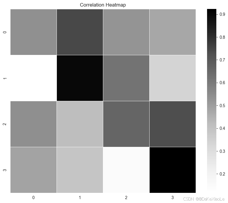
# 输入数据 (生成一个4x4的随机矩阵并展示)。
# 用来生成由此图像变换到target图像的神经网络
input = np.random.rand(4, 4)
# 可视化该图像
show_pic(input)
# 将4x4矩阵展开为16x1列向量
input = input.reshape(-1, 1)
# 初始化第一层隐藏层的权重和偏置
weight0 = np.random.randn(num_hidden_layer0, input.shape[0])  # 16x16权重矩阵
bias0 = np.random.randn(num_hidden_layer0, 1)  # 16x1偏置向量
# 初始化第二层隐藏层的权重和偏置
weight1 = np.random.randn(num_hidden_layer1, num_hidden_layer0)  # 16x16权重矩阵
bias1 = np.random.randn(num_hidden_layer1, 1)  # 16x1偏置向量
# 初始化输出层的权重和偏置
weight2 = np.random.randn(16, num_hidden_layer1)  # 4x16权重矩阵
bias2 = np.random.randn(16, 1)  # 4x1偏置向量

反向传递函数及注释说明
# 反向传播函数
def backpropagation(img, input, weight0, bias0, output0, weight1, bias1, output1, weight2, bias2, output, learning_rate, active_mode):
    # ========================== 输出层梯度计算 ==========================
    # MSE = [(y1 - R1)^2 + (y2 - R2)^2 +……(yn - Rn)^2 ]/n
    # 我们的目标是最小化均方误差 (MSE),Ri为目标值(实际值),yi为模型预测值
    # 所以首先对每个预测值 yi 计算均方误差 MSE 对 yi 的导数
    # d_output_layer = 均方误差(MSE)对模型的预测输出 output 的导数
    # MSE' ~~~mse_loss_derivative~~~> output
    d_output_layer = mse_loss_derivative(output, img) # MSE的导数

    # ========================== 激活函数的导数 ==========================
    # 根据所使用的激活函数(ReLU 或 Sigmoid),计算损失MSE对激活函数输入x的导数
    # 对于 ReLU:ReLU 的导数在输出 > 0 时为 1,输出 <= 0 时为 0
    # 对于 Sigmoid:Sigmoid 的导数为 σ(x)(1 - σ(x)),其中 σ(x) 是 Sigmoid 函数的输出(output)
    # MSE' ~~~mse_loss_derivative~~~> output ~~~ReLU'/Sigmoid'~~~> x
    if active_mode == "ReLU":
        d_output_layer *= (output > 0)  # ReLU 的导数
    else:
        d_output_layer *= output * (1 - output)  # Sigmoid 的导数

    # ========================== 输出层权重和偏置的梯度更新 ==========================
    # 通过链式法则,损失对输出层权重 weight2 和偏置 bias2 的导数可以用 d_output_layer 和上一层的输出计算得出
    # 权重梯度:grad_weight2 = d_output_layer * output1.T
    # 偏置梯度:grad_bias2 = d_output_layer 的累加和
    # x = w1*out1 + w2*out2……wi*outi + b
    # MSE' ~~~mse_loss_derivative~~~> output ~~~ReLU'/Sigmoid'~~~> x ~~~output1i~~~> wi
    # MSE' ~~~mse_loss_derivative~~~> output ~~~ReLU'/Sigmoid'~~~> x ~~~1~~~> wi
    # 其中d_hidden_layer 表示隐藏层2输人x对损失函数的梯度
    grad_weight2 = np.dot(d_output_layer, output1.T)  # 计算输出层权重的梯度
    grad_bias2 = np.sum(d_output_layer, axis=1, keepdims=True)  # 计算输出层偏置的梯度

    # 使用梯度下降法更新输出层的权重和偏置
    weight2 -= learning_rate * grad_weight2  # 更新输出层的权重
    bias2 -= learning_rate * grad_bias2  # 更新输出层的偏置

    # ========================== 隐藏层1的梯度更新 ==========================
    # 通过反向传播计算隐藏层1的梯度
    # d_hidden_layer1 表示隐藏层1输出(output1)对损失函数的梯度
    # 损失函数对隐藏层1的输出导数是通过后续层传递过来的梯度计算得出:
    # d_hidden_layer1 = 修改后的权重 * d_hidden_layer 表示隐藏层2输人x对损失函数的梯度
    # 即 MSE' ~~~mse_loss_derivative~~~> output ~~~ReLU'/Sigmoid'~~~> x ~~~wi~~~> output1i
    # 化简为 MSE' ~~~反向0层~~~> output1
    d_hidden_layer1 = np.dot(weight2.T, d_output_layer)

    # 根据激活函数选择(ReLU 或 Sigmoid)调整隐藏层1的导数
    if active_mode == "ReLU":
        d_hidden_layer1 *= (output1 > 0)  # ReLU 的导数
    else:
        d_hidden_layer1 *= output1 * (1 - output1)  # Sigmoid 的导数

    # ========================== 隐藏层1的权重和偏置更新 ==========================
    # MSE' ~~~反向0层~~~> output1 ~~~ReLU'/Sigmoid'~~~> x ~~~output1i~~~> wi
    # MSE' ~~~反向0层~~~> output1 ~~~ReLU'/Sigmoid'~~~> x ~~~1~~~> wi
    # 计算隐藏层1的权重和偏置的梯度,并使用梯度下降法进行更新
    grad_weight1 = np.dot(d_hidden_layer1, output0.T)  # 计算隐藏层1的权重梯度
    grad_bias1 = np.sum(d_hidden_layer1, axis=1, keepdims=True)  # 计算隐藏层1的偏置梯度

    # 使用梯度下降法更新隐藏层1的权重和偏置
    weight1 -= learning_rate * grad_weight1  # 更新隐藏层1的权重
    bias1 -= learning_rate * grad_bias1  # 更新隐藏层1的偏置

    # ========================== 隐藏层0的梯度更新 ==========================
    # 通过反向传播计算隐藏层0的梯度
    # d_hidden_layer0 表示隐藏层0输出(output0)对损失函数的梯度
    d_hidden_layer0 = np.dot(weight1.T, d_hidden_layer1)

    # 根据激活函数选择(ReLU 或 Sigmoid)调整隐藏层0的导数
    if active_mode == "ReLU":
        d_hidden_layer0 *= (output0 > 0)  # ReLU 的导数
    else:
        d_hidden_layer0 *= output0 * (1 - output0)  # Sigmoid 的导数

    # ========================== 隐藏层0的权重和偏置更新 ==========================
    # 计算隐藏层0的权重和偏置的梯度,并使用梯度下降法进行更新
    grad_weight0 = np.dot(d_hidden_layer0, input.T)  # 计算隐藏层0的权重梯度
    grad_bias0 = np.sum(d_hidden_layer0, axis=1, keepdims=True)  # 计算隐藏层0的偏置梯度

    # 使用梯度下降法更新隐藏层0的权重和偏置
    weight0 -= learning_rate * grad_weight0  # 更新隐藏层0的权重
    bias0 -= learning_rate * grad_bias0  # 更新隐藏层0的偏置

    # 返回更新后的权重和偏置
    return weight0, bias0, weight1, bias1, weight2, bias2
前向传播函数及注释说明
# 前向传播函数
def forward(input, weight0, bias0, weight1, bias1, weight2, bias2, active_mode):
    # 计算各层的输出
    output0 = ReLU(np.dot(weight0, input) + bias0) if active_mode == "ReLU" else sigmoid(np.dot(weight0, input) + bias0)
    output1 = ReLU(np.dot(weight1, output0) + bias1) if active_mode == "ReLU" else sigmoid(np.dot(weight1, output0) + bias1)
    output = ReLU(np.dot(weight2, output1) + bias2) if active_mode == "ReLU" else sigmoid(np.dot(weight2, output1) + bias2)

    return output0, output1, output
进入循环体
# 计算初始损失
img = img.reshape(-1, 1)
loss = mse_loss(input, img)
print("Initial loss:", loss)
# 训练过程
output0, output1, output = forward(input, weight0, bias0, weight1, bias1, weight2, bias2, active_mode)
for i in range(times +1):
    # 反向传播
    weight0, bias0, weight1, bias1, weight2, bias2 = backpropagation(img, input, weight0, bias0, output0, weight1, bias1, output1, weight2, bias2, output, learning_rate, active_mode)
    # 前向传播
    output0, output1, output = forward(input, weight0, bias0, weight1, bias1, weight2, bias2, active_mode)

    # 添加图像到 TensorBoard 中 (注意要调整通道维度)
    image_np = show(output.reshape(-1, 4))
    writer.add_image('Heatmap', image_np.transpose(2, 0, 1), i)  # 确保图像的通道为 (C, H, W)

    # 计算并打印更新后的损失
    new_loss = mse_loss(output, img)
    print(f"Step {i}: Loss = {new_loss}")

# 关闭 TensorBoard 日志记录器
writer.close()
# 可视化该图像
show_pic(output.reshape(-1, 4))
TensorBoard 保存并展示训练过程中的输出图像。
在新的locatio中输入,启动TensorBoard
tensorboard --logdir=logs
Serving TensorBoard on localhost; to expose to the network, use a proxy or pass --bind_all
TensorBoard 2.18.0 at http://localhost:6006/ (Press CTRL+C to quit)
通过浏览器打开
结果参考绑定资源


 1万+
1万+

 被折叠的 条评论
为什么被折叠?
被折叠的 条评论
为什么被折叠?
 到【灌水乐园】发言


