2D/3D 中弗里德里希常数和庞加莱常数的计算（Matlab代码实现）

 💥💥💞💞欢迎来到本博客❤️❤️💥💥

🏆博主优势：🌞🌞🌞博客内容尽量做到思维缜密，逻辑清晰，为了方便读者。

⛳️座右铭：行百里者，半于九十。

目录

💥1 概述

📚2 运行结果

2D

3D

🎉3 参考文献

🌈4 Matlab代码实现

💥1 概述

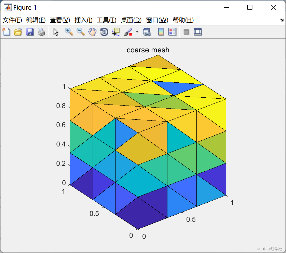
质量和刚度矩阵被组装成嵌套的均匀网格（2D 中的三角形和 3D 中的四面体），从具有少量元素的粗网格（level=1 网格）开始，到具有多达数百万元素的最精细网格（level=levels，其中级别是预定义的），具体取决于可用内存。

弗里德里希、庞加莱是从广义特征值问题近似出来的。如果已知，则将近似值与精确值进行比较（例如，对于 2D 中的矩形域和 3D 中的长方体域），并可视化相应的特征函数。域几何可以通过修改输入矩阵轻松更改：node2coords，elems2nodes，dirichlet。还有一个麦克斯韦常数的实验计算。本文解释的弗里德里希常数的原始计算。

📚2 运行结果

2D

 

 

 

 

 

3D

 

 部分代码：

d=2;   %problem dimension

levels=5;   %level=9 uniform refinement leading to elements=524288, edges=787456, nodes=263169 triagulation for the unit square problem
level_visualize=3; 

levels_CF=levels;   %level uniform refinement for the Friedrichs constant
levels_CP=levels;   %level uniform refinement for the Poincare constant      
levels_CM=0*levels;   %level uniform refinement for the Maxwell constant, set zero to switch off this computation

level_visualize_eigenfunctionF=min(levels_CF,level_visualize);
level_visualize_eigenfunctionP=min(levels_CP,level_visualize);
level_visualize_eigenfunctionM=min(levels_CM,level_visualize);

if ~exist('levels')
    levels=max(max(levels_CF,levels_CP),levels_CM);
end

fprintf('The last level of uniform refinement is %d. ', levels);
fprintf('Please wait for all levels. \n');
fprintf('\n');

   
switch model
    case 'rectangle'
        a=1; b=1;                           %rectangle lengths       
        %coarse mesh of the unit square
        nodes2coord = 0.5*[0 0; 1 0; 2 0; 2 1; 1 1; 0 1; 0 2; 1 2; 2 2];
        elems2nodes = [1 2 5; 5 6 1; 2 3 4; 2 4 5; 6 5 8; 6 8 7; 5 4 9; 5 9 8];
        dirichlet   = [1 2; 2 3; 3 4; 4 9; 9 8; 8 7; 7 6; 6 1];    
        nodes2coord(:,1)=nodes2coord(:,1)*a;  
        nodes2coord(:,2)=nodes2coord(:,2)*b;
        
        [nodes2coord,elems2nodes,dirichlet] = refinement_uniform_2D(nodes2coord,elems2nodes,dirichlet);

        ab=[a,b];                                             %max(max(nodes2coord,1))-min(min(nodes2coord,1));
        CF_exact=sum((pi./ab).^2)^(-1/2);                     %exact value of the Fridrichs constant for rectangle a x b
        CP_exact=max(ab)/pi;                                  %exact value of the Poincare constant
        CM_exact=CF_exact;                                    %exact value of the Maxwell constant (with zero normal bc) if available

    case 'Lshape'
        %switching back to Lshape as in the first paper
        nodes2coord = 0.5*[0 0; 1 0; 2 0; 2 1; 1 1; 0 1; 0 2; 1 2];
        elems2nodes = [1 2 5; 5 6 1; 2 3 4; 2 4 5; 6 5 8; 6 8 7];
        dirichlet   = [1 2; 2 3; 3 4; 4 5; 5 8; 8 7; 7 6; 6 1];
        [nodes2coord,elems2nodes,dirichlet] = refinement_uniform_2D(nodes2coord,elems2nodes,dirichlet);
        
    case 'annulus'  
        a=0.5; b=2; L=2; N=10;       
        [elems2nodes,nodes2coord,~,~,outer_boundary,inner_boundary]=get_ring_data(a,b,N,L);
        dirichlet=[outer_boundary; inner_boundary];    
end

figure; show_mesh(elems2nodes,nodes2coord); xlabel('x'); ylabel('y'); axis image; enlarge_axis(0.1,0.1); title('coarse mesh');
if printout
    prepare_to_print; print('-painters','-dpdf','mesh_coarse');
end

level_nodes = zeros(levels,1);
level_edges = zeros(levels,1);
level_CF=zeros(levels_CF,1);
level_CP=zeros(levels_CP,1);
level_CM=zeros(levels_CM,1);
%level_CM_zeroEigenvalueMultiplicity=zeros(levels,1);

for level=1:levels
    % uniform refinement
    if (level>1)
        if strcmp(model,'annulus')
            N=N*2; L=L*2;
            [elems2nodes,nodes2coord,~,~,outer_boundary,inner_boundary]=get_ring_data(a,b,N,L);
            dirichlet=[outer_boundary; inner_boundary]; 
        else
            [nodes2coord,elems2nodes,dirichlet] = refinement_uniform_2D(nodes2coord,elems2nodes,dirichlet);
        end
    end

    % affine transformations
    [B_K,~,B_K_det] = affine_transformations(nodes2coord,elems2nodes);
    
    % edgewise data for Nedelec0 and RT0 element
    elems2edges = get_edges(elems2nodes);
    signs = signs_edges(elems2nodes);
    
    assembly_all_matrices;
    
    dirichlet_nodes=unique(dirichlet);
    
    compute_constants; 
    
    visualize_eigenfunctions;  
    
    if level==level_visualize
       figure; show_mesh(elems2nodes,nodes2coord); xlabel('x'); ylabel('y'); axis image; enlarge_axis(0.1,0.1); title('fine mesh');
       if printout
           prepare_to_print; print('-painters','-dpdf','mesh_fine');
       end
    end
end

visualize_constants;

if strcmp(model,'rectangle')
    test_wave
end

🎉3 参考文献

部分理论来源于网络，如有侵权请联系删除。

[1] Jan Valdman, Minimization of Functional Majorant in A Posteriori Error Analysis based on H(div) Multigrid-Preconditioned CG Method, Advances in Numerical Analysis, vol. 2009, Article ID 164519 (2009)

[2] Talal Rahman, Jan Valdman, Fast MATLAB assembly of FEM matrices in 2D and 3D: nodal elements. Applied Mathematics and Computation 219, 7151–7158 (2013)

[3] Immanuel Anjam, Jan Valdman, Fast MATLAB assembly of FEM matrices in 2D and 3D: Edge elements. Applied Mathematics and Computation 267, 252–263 (2015)

🌈4 Matlab代码实现