PyTorch--用Variable实现线性回归

最新推荐文章于 2025-12-03 23:35:39 发布

原创最新推荐文章于 2025-12-03 23:35:39 发布 · 519 阅读

0 ·

CC 4.0 BY-SA版权

文章标签：

#pytorch #线性回归 #python

深度学习与PyTorch 专栏收录该内容

3 篇文章

订阅专栏

本文通过使用PyTorch的autograd模块实现了一个简单的线性回归模型，并演示了如何通过迭代更新权重和偏差来最小化损失函数。通过可视化的手段展示了训练过程中的预测结果与真实数据之间的对比。

部署运行你感兴趣的模型镜像

PyTorch–用Variable实现线性回归

从中体会autograd的便捷之处

1.导入库

import torch as t
from torch.autograd import Variable as V
from matplotlib import pyplot as plt
from IPython import display

2.定义函数

#为了在不同的计算机运行一样，设置随机种子
t.manual_seed(1000)

def get_fake_data(batch_size=8):
    x = t.rand(batch_size, 1) * 20
    y = x * 2 + (1 + t.randn(batch_size, 1)) * 3
    return x, y

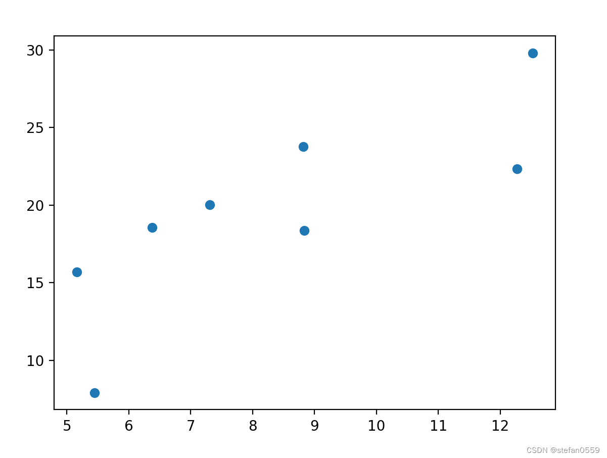
3.查看分布

x, y = get_fake_data()
plt.scatter(x.squeeze().numpy(), y.squeeze().numpy())

如下图
在这里插入图片描述

4.网络设计及画图

#随机初始化参数
w = V(t.rand(1, 1), requires_grad=True)
b = V(t.zeros(1, 1), requires_grad=True)
lr = 0.001

for i in range(8000):
    x, y =get_fake_data()
    x, y = V(x), V(y)
    #forward
    y_pred = x.mm(w) + b
    loss = 0.5 * (y_pred - y) ** 2
    loss = loss.sum()

    #backward
    loss.backward()
    #更新参数
    w.data.sub_(lr * w.grad.data)
    b.data.sub_(lr * b.grad.data)
    #梯度清零
    w.grad.data.zero_()
    b.grad.data.zero_()

    if i % 2000 == 0:
        display.clear_output(wait=True)
        x = t.arange(0, 20, dtype=t.float).view(-1, 1)
        y = x.mm(w.data) + b.expand_as(x)
        plt.plot(x.detach().numpy(), y.detach().numpy())#predicted

        x2, y2 = get_fake_data(batch_size=20)
        plt.scatter(x2.numpy(), y2.numpy())#true data

        plt.xlim(0, 20)
        plt.ylim(0, 40)
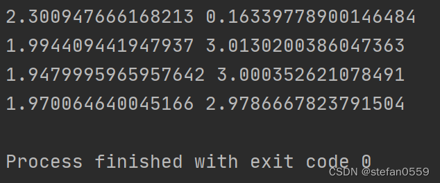
        print(w.item(), b.item())
        plt.show()

图如下
在这里插入图片描述
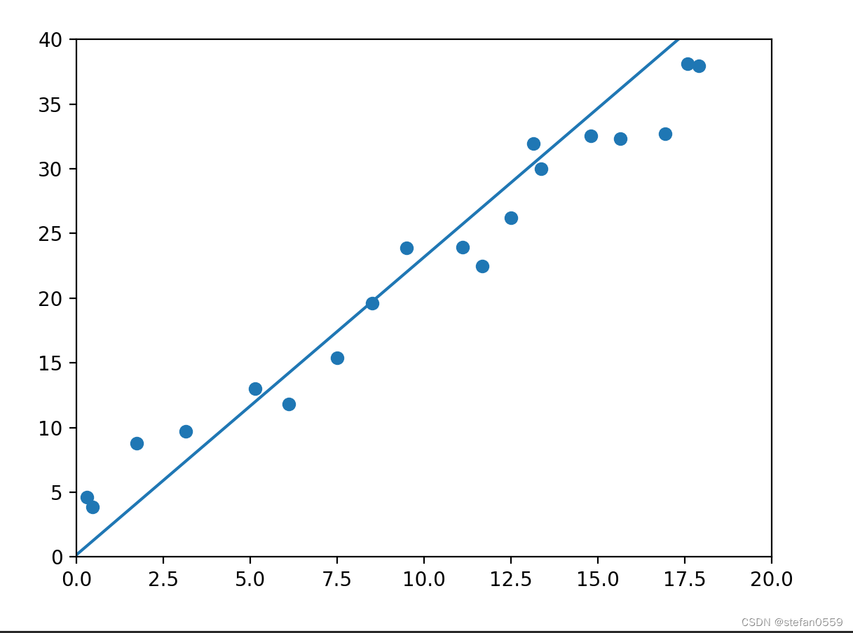
相关参数值

您可能感兴趣的与本文相关的镜像

PyTorch 2.5

PyTorch

Cuda

PyTorch 是一个开源的 Python 机器学习库，基于 Torch 库，底层由 C++ 实现，应用于人工智能领域，如计算机视觉和自然语言处理