MATLAB基础笔记7 统计和数据分析 / 曲线拟合和插值

MATLAB统计与数据分析

最新推荐文章于 2023-11-16 21:03:08 发布

原创最新推荐文章于 2023-11-16 21:03:08 发布 · 874 阅读

5 ·

CC 4.0 BY-SA版权

文章标签：

#matlab #数学建模 #数据分析 #统计学

笔记同时被 2 个专栏收录

34 篇文章

订阅专栏

matlab

7 篇文章

订阅专栏

本文介绍了MATLAB在统计和数据分析中的应用，包括算术平均、中位数、众数、四分位数的计算，箱线图绘制，偏态分析，双样本t检验，以及一维和二维数据的曲线拟合和插值方法。通过实例展示了如何使用MATLAB进行数据的统计描述、假设检验和数据建模。

MATLAB笔记7 统计和数据分析 / 曲线拟合和插值

统计操作

Mean算术平均, Median中位数, Mode中位数, and Quartile四分位数

>> load stockreturns;
x4 = stocks(:,4);
>> mean(x4)

ans =

  -5.8728e-04

>> median(x4)

ans =

    0.0617

>> mode(x4)

ans =

   -5.8764

>> quantile(x4,0.25,1)

ans =

   -1.5082

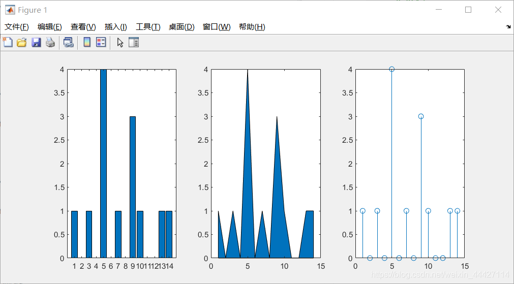
画图

x = 1:14;
freqy = [1 0 1 0 4 0 1 0 3 1 0 0 1 1];
subplot(1,3,1); bar(x,freqy); xlim([0 15]);
subplot(1,3,2); area(x,freqy); xlim([0 15]);
subplot(1,3,3); stem(x,freqy); xlim([0 15]);

在这里插入图片描述

箱线图

>> marks = [80 81 81 84 88 92 92 94 96 97];
boxplot(marks)
prctile(marks, [25 50 75])

ans =

    81    90    94

在这里插入图片描述

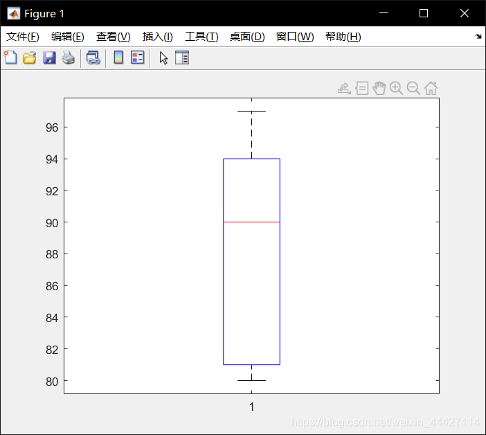
boxplot 画箱线图， prctile获得分位数

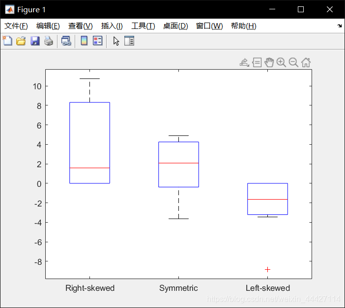
Skewness偏态 skewness()

>> X = randn([10 3])*3;
X(X(:,1)<0, 1) = 0; X(X(:,3)>0, 3) = 0;
boxplot(X, {'Right-skewed', 'Symmetric', 'Left-skewed'});
y = skewness(X)

y =

    0.8167   -0.6878   -1.5176

在这里插入图片描述

统计假设检验

ttest2() 双样本 t 检验
h = ttest2(x,y) 使用双样本 t 检验返回原假设的检验决策，该原假设假定向量 x 和 y 中的数据来自均值相等、方差相同但未知的正态分布的独立随机样本。备择假设是 x 和 y 中的数据来自均值不相等的总体。如果检验在 5% 的显著性水平上拒绝原假设，则结果 h 为 1，否则为 0。

以下例子测试两个样本均值是否相等

>> load stockreturns;
x1 = stocks(:,3); x2 = stocks(:,10);
boxplot([x1, x2], {'3', '10'});
[h,p] = ttest2(x1, x2)

h =

     1


p =

    0.0423

h=1，故拒绝原假设：x1和x2样本的均值相等；显著水平为5%，而p=0.0423<0.05

曲线拟合

polyfit()

>> x =[-1.2 -0.5 0.3 0.9 1.8 2.6 3.0 3.5];
y =[-15.6 -8.5 2.2 4.5 6.6 8.2 8.9 10.0];
fit = polyfit(x,y,1);

要进行拟合的散点为（-1.2，-15.6），（-0.5，-8.5）…
polyfit第三参数为1表示用一次函数拟合
函数返回ax+b中的a，b值

>> xfit = [x(1):0.1:x(end)]; yfit = fit(1)*xfit + fit(2);
plot(x,y,'ro',xfit,yfit,'b'); set(gca,'FontSize',14);
legend('data points','best-fit','location','northwest');

在这里插入图片描述

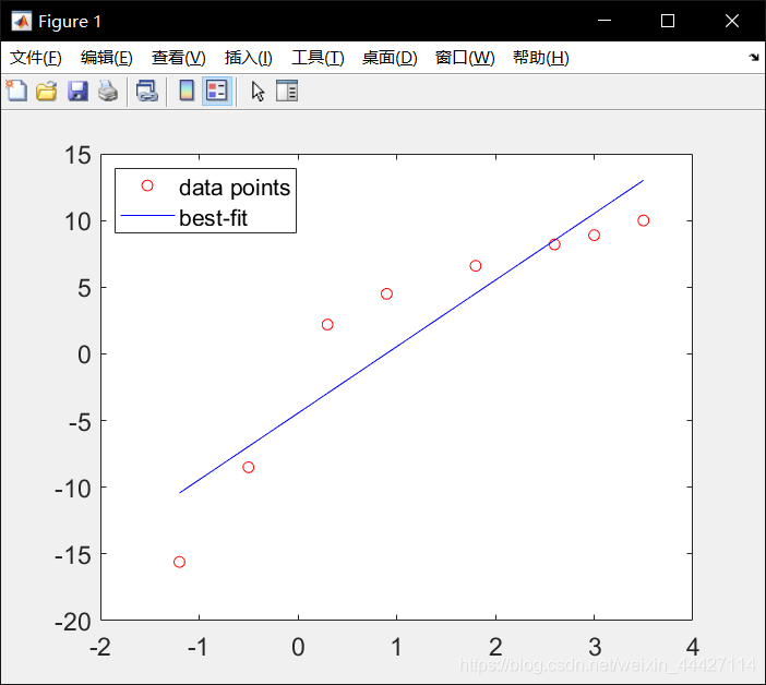
yfit = fit(1)*xfit + fit(2) 表示用一次拟合函数 y=ax+b 拟合

corrcoef() 求相关系数

相关系数 −1 ≤ 𝑟 ≤ 1，越接近于 1 则接近正相关，越接近 -1 则接近负相关

依然是上面的数据，判断 xy 的相关性

>> x =[-1.2 -0.5 0.3 0.9 1.8 2.6 3.0 3.5];
y =[-15.6 -8.5 2.2 4.5 6.6 8.2 8.9 10.0];
scatter(x,y); box on; axis square;
corrcoef(x,y)

ans =

    1.0000    0.9202
    0.9202    1.0000

相关系数为0.9202接近 1，为正相关
scatter() 功能为画散点图，也称气泡图（点是一个一个圈圈 ooooooo）

高阶多项式拟合

>> x =[-1.2 -0.5 0.3 0.9 1.8 2.6 3.0 3.5];
y =[-15.6 -8.5 2.2 4.5 6.6 8.2 8.9 10.0];
figure('Position', [50 50 1500 400]);
for i=1:3
    subplot(1,3,i); p = polyfit(x,y,i);
    xfit = x(1):0.1:x(end); yfit = polyval(p,xfit);
    plot(x,y,'ro',xfit,yfit,'b'); set(gca,'FontSize',14);
    ylim([-17, 11]); legend('Data points','Fitted curve','location','southeast');
end

在这里插入图片描述

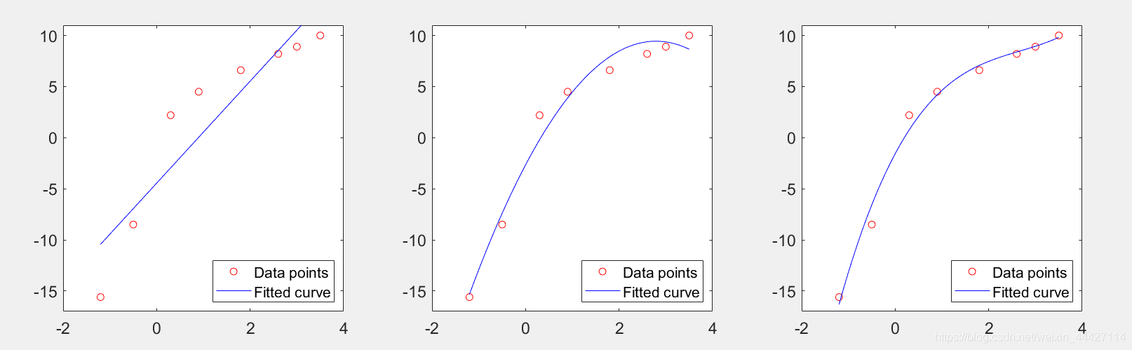
越高阶不一定拟合的越好，可能会过拟合

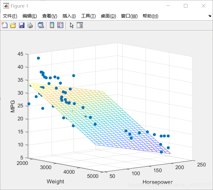
regress() 多变量的函数拟合
拟合函数形如：𝑦 = 𝛽0 + 𝛽1𝑥1 + 𝛽2𝑥2

load carsmall;
y = MPG;
x1 = Weight; x2 = Horsepower;
X = [ones(length(x1),1) x1 x2];
b = regress(y,X);
x1fit = min(x1):100:max(x1);
x2fit = min(x2):10:max(x2);
[X1FIT,X2FIT]=meshgrid(x1fit,x2fit);
YFIT=b(1)+b(2)*X1FIT+b(3)*X2FIT;
scatter3(x1,x2,y,'filled'); hold on;
mesh(X1FIT,X2FIT,YFIT); hold off;
xlabel('Weight');
ylabel('Horsepower');
zlabel('MPG'); view(50,10);

在这里插入图片描述

另一用法：[b,bint,r,rint,stats]=regress(y,X);
如果方程非线性用 Curve Fitting Toolbox: cftool() 即曲线拟合工具箱:cftool()；matlab输入 cftool 或 cftool()

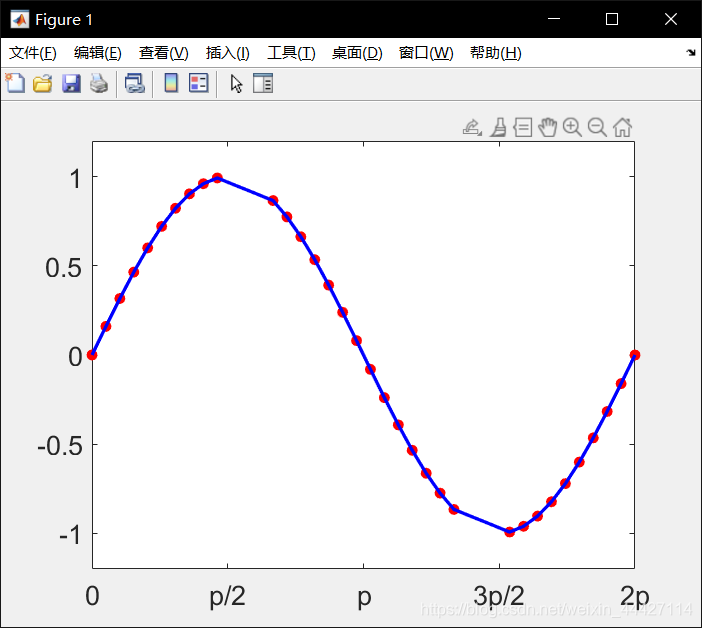
Interpolation 插值

interp1() 线性插值

x = linspace(0, 2*pi, 40); 
x_m = x;
x_m([11:13, 28:30]) = NaN; 
y_m = sin(x_m);
hold on;
plot(x_m, y_m,'ro', 'MarkerFaceColor', 'r');
xlim([0, 2*pi]); 
ylim([-1.2, 1.2]); 
box on;   %显示坐标区轮廓
set(gca, 'FontName', 'yahei', 'FontSize', 16);
set(gca, 'XTick', 0:pi/2:2*pi);
set(gca, 'XTickLabel', {'0', 'p/2', 'p', '3p/2', '2p'});
m_i = ~isnan(x_m);
y_i = interp1(x_m(m_i), ...
y_m(m_i), x);
plot(x,y_i,'-b', ...
'LineWidth', 2);
hold off;

在这里插入图片描述

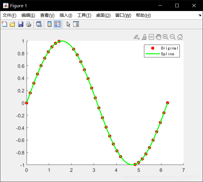
spline() 样条插值

m_i = ~isnan(x_m);
y_i = spline(x_m(m_i), y_m(m_i), x);
hold on; 
plot(x_m, y_m,'ro', 'MarkerFaceColor', 'r');
plot(x,y_i,'-g', 'LineWidth', 2); 
hold off;
h = legend('Original', 'Spline');
set(h,'FontName', 'kaiti');

在这里插入图片描述

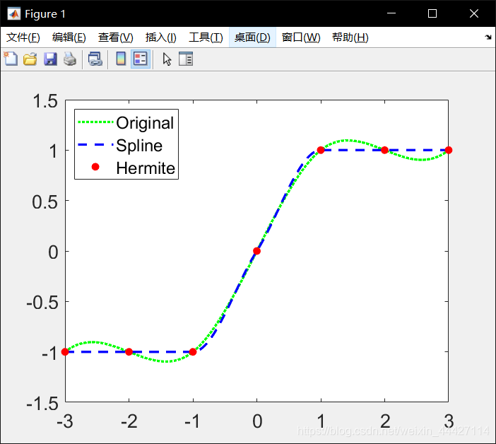
三次样条插值和 Hermite 多项式

x = -3:3; 
y = [-1 -1 -1 0 1 1 1]; 
t = -3:.01:3;
s = spline(x,y,t); 
p = pchip(x,y,t);
hold on; 
plot(t,s,':g', 'LineWidth', 2);
plot(t,p,'--b', 'LineWidth', 2);
plot(x,y,'ro', 'MarkerFaceColor', 'r');
hold off; 
box on; 
set(gca, 'FontSize', 16);
h = legend(2,'Original', 'Spline', 'Hermite');

在这里插入图片描述

interp2() meshgrid 格式的二维网格数据的插值

xx = -2:.5:2; 
yy = -2:.5:3;
[X,Y] = meshgrid(xx,yy);
Z = X.*exp(-X.^2-Y.^2);
surf(X,Y,Z); hold on;
plot3(X,Y,Z+0.01,'ok','MarkerFaceColor','r')

xx_i = -2:.1:2; 
yy_i = -2:.1:3;
[X_i,Y_i] = meshgrid(xx_i,yy_i);
Z_i = interp2(xx,yy,Z,X_i,Y_i);
surf(X_i,Y_i,Z_i); hold on;
plot3(X,Y,Z+0.01,'ok','MarkerFaceColor','r')

样条二维插值

xx = -2:.5:2; 
yy = -2:.5:3; 
[X,Y] = meshgrid(xx,yy);
Z = X.*exp(-X.^2-Y.^2); 
xx_i = -2:.1:2; 
yy_i = -2:.1:3;
[X_i,Y_i] = meshgrid(xx_i,yy_i);
Z_c = interp2(xx,yy,Z,X_i,Y_i,'cubic');
surf(X_i,Y_i,Z_c); 
hold on;
plot3(X,Y,Z+0.01,'ok', 'MarkerFaceColor','r');
hold off;