


 这篇博客主要介绍了Python在数据统计和可视化方面的应用,包括基本数据统计如便捷数据获取、数据准备、显示、选择和简单统计,以及高级数据处理如聚类分析。同时,讲解了matplotlib库的绘图基础和图像属性控制,以及使用pandas进行数据可视化的方法。此外,还探讨了python在理工科和人文社科领域的具体应用。
05_python数据统计和可视化
01_4-1 python基本数据统计
01_1-便捷数据获取
# 用python获取数据:本地数据获取(文件的打开、读写和关闭);网络数据获取(抓取网页,解析网页内容,urllib,urllib2,httplib,httplib2)
# 便捷网络数据
from matplotlib.finance import quotes_historical_yahoo_ochl
from datetime import date
import pandas as pd
today = date.today()
print (today)
start = (today.year-1,today.month,today.day)
# quotes = quotes_historical_yahoo_ochl ('CCE',start,today)
quotes = quotes_historical_yahoo_ochl('AXP', start, today)
df = pd.DataFrame(quotes)
print (df)
# 自然语言工具包 NLTK:古腾堡语料库,布朗语料库,路透社语料库,网络和聊天文本……
from nltk.corpus import gutenberg
import nltk
print (gutenberg.fileids())
02_2数据准备
# 数据整理
from matplotlib.finance import quotes_historical_yahoo_ochl
from datetime import date
import pandas as pd
today = date.today()
print (today)
start = (today.year-1,today.month,today.day)
# quotes = quotes_historical_yahoo_ochl ('CCE',start,today)
quotes = quotes_historical_yahoo_ochl('AMX', start, today)
fileds = ['date','open','close','high','low','volume']
df = pd.DataFrame(quotes,columns = fields)
print (df)
# 数据整理
from datetime import date
a = date.fromordinal(735190)
print (a)
2013-11-18
# 创建时间序列
import pandas as pd
dates = pd.date_range('20141001',periods=7)
print (dates)

import numpy as np
dates = pd.DataFrame(np.random.randn(7,3),index = dates,columns=list('ABC'))
print (dates)
DatetimeIndex(['2014-10-01', '2014-10-02', '2014-10-03', '2014-10-04',
               '2014-10-05', '2014-10-06', '2014-10-07'],
              dtype='datetime64[ns]', freq='D')
                   A         B         C
2014-10-01 -0.671403 -0.218888  0.238439
2014-10-02 -0.305552 -2.049908  1.416983
2014-10-03  0.438262 -0.892854  0.121548
2014-10-04 -0.966557 -0.784305 -1.017663
2014-10-05  0.882889  1.418623 -0.927695
2014-10-06 -1.236913  0.638172 -0.379498
2014-10-07  1.077244 -0.664185 -0.372371
03_3 数据显示
# 数据显示
# 显示方式:显示索引,显示列名,显示数据的值,显示数据描述
# a.index  a.columns a.values a.describe
# 索引的格式:quotesdf.index
# 显示行:专用方式;切片
# df.head[5] = df[:5]
# df.tail[5] = df[25:]
04_4数据选择
# 选择方式:选择行,选择列,选择区域,筛选(条件选择)
# 选规行:切片,索引,quotesdf[u'2013-12-02':u'2013-12-06']
# 选择列:列名,djidf['code'],djidf.code
# 选择方式:行、列 标签label(loc)  djidf.loc[1:5] djidf.loc[:['code','lasttrade']]
# 行和列的区域:标签label(loc);单个值(at)djidf.loc[1:5,['code','lasttrade']]   djidf.loc[1,lasttrade'] djidf.at[1,lasttrade']
# 行、列和区域:用iloc(位置);取某个值(iat) djidf.iloc[1:6,[0,2]] djidf.iloc[1,2] djidf.iat[1,2]
# 条件筛选 quotesdf[quotesdf.index>=u'2014-01-01'] quotesdf[(quotesdf.index>=u'2014-01-01')&(quotesdf.close>=95)]
05_5简单统计与筛选
# 最近一次成交价的平均值 djidf.mean(columns = 'lasttrade')
# 最近一次成交价大于等于120的公司名 djidf[djidf.lasttrade >= 120].name
# 统计股票涨和跌的天数 len(quotesdf[quotesdf.close > quotesdf.open])
# 统计相邻两天收盘价的涨跌情况 s=(np.sign(np.diff(quotesdf.close)) s[np.where(s == 1)].size s[np.where(s == -1)].size
# 排序 djidf.sort(columns = 'lasttrade')  djidf.sort(columns = 'lasttrade')[27:].name
# 计数统计 统计2014年1月份的股票开盘天数 t= quotesdf[(quotesdf.index >= '2014-01-01')&(quotesdf.index < '2014-02-01')]
06_6-grouping
# 统计近一年每个月的股票开盘天数 tempdf.groupby('month').count()  tempdf.groupby('month').count().month
# 统计近一年每个月的总成交量 tempdf.groupby('month').sum().volume
# 更高效的统计近一年每个月的总成交量 g = tempdf.groupby('month')  gvolume = g['volume']  print(gvolume.sum())
07_7-merge
# append
# p = quotesdf[:2] q = quotesdf[u'2014-01-01':u'2014-01-05'] p.append(q)
# concat 将前五个数据和后五个数据合并
# pieces = [tempdf[:5],tempdf[len(tempdf)-4:]] pd.concat(pieces)
# 连接两个不同逻辑结构的对象  piece1 = quotesdf[:3] piece2=tempdf[:3] pd.concat([piece1,piece2],ignore_index = True)
# objs join keys names ignore_index axis join_axes levels verify_integrity
# join
# pd.merge(djidf,AKdf,on = 'code')  pd.merge(djidf,AKdf, on = 'code').drop(['lasttrade'],axis = 1)
# left right how on left_on right_on left_index right_index sort suffixes copy
print (list(range(12,3,-1)))
[12, 11, 10, 9, 8, 7, 6, 5, 4]
02_4-2-python高级数据处理与可视化
01_1聚类分析
from pylab import *
from scipy.cluster.vq import *
# from scipy import *
list1 = [88.0,74,96,85]
list2 = [92,99,95,94]
list3 = [91,87,99,95]
list4 = [78,99,97,81]
list5 = [88,78,98,84]
list6 = [100,95,100,92]
data = np.vstack((list1,list2,list3,list4,list5,list6))
centroids,_=kmeans(data,2)
result,_ =vq(data,centroids)
print (result)
[0 1 1 1 0 1]
help (kmeans)
Help on function kmeans in module scipy.cluster.vq:

kmeans(obs, k_or_guess, iter=20, thresh=1e-05, check_finite=True)
    Performs k-means on a set of observation vectors forming k clusters.

    The k-means algorithm adjusts the centroids until sufficient
    progress cannot be made, i.e. the change in distortion since
    the last iteration is less than some threshold. This yields
    a code book mapping centroids to codes and vice versa.

    Distortion is defined as the sum of the squared differences
    between the observations and the corresponding centroid.

    Parameters
    ----------
    obs : ndarray
       Each row of the M by N array is an observation vector. The
       columns are the features seen during each observation.
       The features must be whitened first with the `whiten` function.

    k_or_guess : int or ndarray
       The number of centroids to generate. A code is assigned to
       each centroid, which is also the row index of the centroid
       in the code_book matrix generated.

       The initial k centroids are chosen by randomly selecting
       observations from the observation matrix. Alternatively,
       passing a k by N array specifies the initial k centroids.

    iter : int, optional
       The number of times to run k-means, returning the codebook
       with the lowest distortion. This argument is ignored if
       initial centroids are specified with an array for the
       ``k_or_guess`` parameter. This parameter does not represent the
       number of iterations of the k-means algorithm.

    thresh : float, optional
       Terminates the k-means algorithm if the change in
       distortion since the last k-means iteration is less than
       or equal to thresh.

    check_finite : bool, optional
        Whether to check that the input matrices contain only finite numbers.
        Disabling may give a performance gain, but may result in problems
        (crashes, non-termination) if the inputs do contain infinities or NaNs.
        Default: True

    Returns
    -------
    codebook : ndarray
       A k by N array of k centroids. The i'th centroid
       codebook[i] is represented with the code i. The centroids
       and codes generated represent the lowest distortion seen,
       not necessarily the globally minimal distortion.

    distortion : float
       The distortion between the observations passed and the
       centroids generated.

    See Also
    --------
    kmeans2 : a different implementation of k-means clustering
       with more methods for generating initial centroids but without
       using a distortion change threshold as a stopping criterion.

    whiten : must be called prior to passing an observation matrix
       to kmeans.

    Examples
    --------
    >>> from numpy import array
    >>> from scipy.cluster.vq import vq, kmeans, whiten
    >>> features  = array([[ 1.9,2.3],
    ...                    [ 1.5,2.5],
    ...                    [ 0.8,0.6],
    ...                    [ 0.4,1.8],
    ...                    [ 0.1,0.1],
    ...                    [ 0.2,1.8],
    ...                    [ 2.0,0.5],
    ...                    [ 0.3,1.5],
    ...                    [ 1.0,1.0]])
    >>> whitened = whiten(features)
    >>> book = np.array((whitened[0],whitened[2]))
    >>> kmeans(whitened,book)
    (array([[ 2.3110306 ,  2.86287398],    # random
           [ 0.93218041,  1.24398691]]), 0.85684700941625547)

    >>> from numpy import random
    >>> random.seed((1000,2000))
    >>> codes = 3
    >>> kmeans(whitened,codes)
    (array([[ 2.3110306 ,  2.86287398],    # random
           [ 1.32544402,  0.65607529],
           [ 0.40782893,  2.02786907]]), 0.5196582527686241)
03_3 matplotlib绘图基础
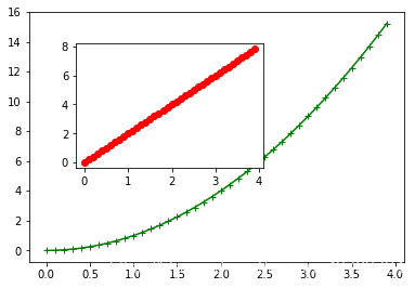
# matplotlib主要用于二位绘图,画图质量高,方便快捷的绘图模块:绘图API——pyplot模块;集成库——pylab模块(包含numpy和pyplot中的常用函数)
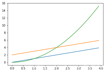
import numpy as np
import matplotlib.pyplot as plt
t = np.arange(0.,4.,0.1)
plt.plot(t,t,t,t+2,t,t**2)
plt.show()
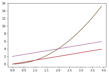
import numpy as np
import pylab as pl
t = np.arange(0,4,0.1)
pl.plot(t,t,t,t+2,t,t**2)
plt.show()
03_3 matplotlib 图像属性控制
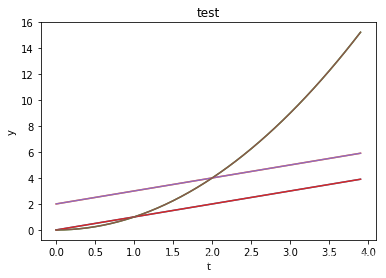
import numpy as np
import matplotlib.pyplot as plt
t = np.arange(0.,4.,0.1)
plt.plot(t,t,t,t+2,t,t**2)
plt.title('test')
plt.xlabel('t')
plt.ylabel('y')
plt.show()
import numpy as np
import pylab as pl
pl.figure(figsize=(8,6),dpi=100)
t = np.arange(0,4,0.1)
pl.plot(t,t,color='red',linestyle='-',linewidth=3,label='line 1')
pl.plot(t,t+2,color='green',linestyle='',marker='*',linewidth=3,label='line 2')
pl.plot(t,t**2,color='blue',linestyle='',marker='+',linewidth=3,label='line 3')
pl.legend(loc='best')#'upper right', 'upper left', 'lower left', 'lower right', 'right', 'center left', 'center right', 'lower center', 'upper center', 'center'
pl.show()

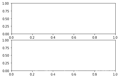
#子图-subplots
plt.subplot(2,1,1)
plt.subplot(2,1,2)
plt.show()
#子图-axes axes([left,bottom,width,height])
import numpy as np
import matplotlib.pyplot as plt
t = np.arange(0,4,0.1)
plt.axes([0.1,0.1,0.8,0.8])
plt.plot(t,t**2,color = 'green',marker='+')
plt.axes([0.2,0.4,0.4,0.4])
plt.plot(t,t*2,color = 'r',marker='o')
plt.show()
04_4pandas 作图
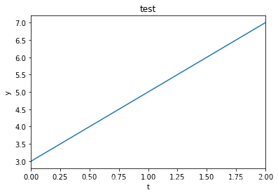
# Pandas通过整合matplotlib的相关功能,可以实现基于series和dataframe的某些绘图功能,针对这两种类型的数据,pandas作图会比pyplot,pylab更方便。
# Pandas可以直接对series和dataframe绘图,更加方便,更加有效。
import pandas as pd
import numpy as np
t = pd.Series([3,5,7])
print(t)
t.plot()
plt.title('test')
plt.xlabel('t')
plt.ylabel('y')
plt.show()
0    3
1    5
2    7
dtype: int64
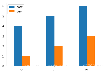
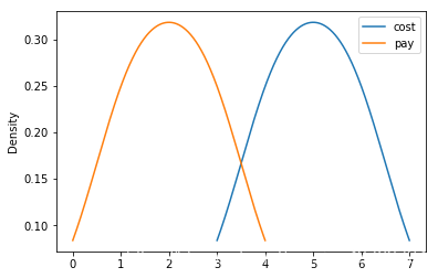
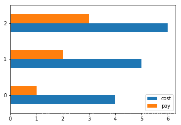
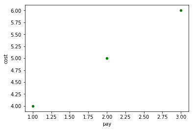
# pandas控制图像形式
data = {'pay':[1,2,3],'cost':[4,5,6]}
a = pd.DataFrame(data)
print(a)
a.plot(kind = 'bar')
a.plot(kind = 'kde')
a.plot(kind = 'barh')
a.plot(kind = 'scatter',x='pay',color='g',y='cost')
plt.show()
   cost  pay
0     4    1
1     5    2
2     6    3
05_5-数据处理
# csv格式数据存取,可以用excel 和 记事本打开
# .csv可以以纯文本形式存储表格数据,可以保存若干个记录,每条记录中的数据之间用逗号来分割。是逗号分隔值的三个单词的缩写。
from matplotlib,finance import quotes_historical_yahoo
from datatime import date
import pandas as pd
today = date.today()
start = (today.year-1,today.month,today.day)
quotes = quotes_historical_yahoo('IBM',start,today)
df = pd.DataFrame(quotes)
df.to_csv('1.csv')

result = pd.read_csv('1.csv')
print(result)
print(result['2'])
# xls格式数据存取
from matplotlib,finance import quotes_historical_yahoo
from datatime import date
import pandas as pd
today = date.today()
start = (today.year-1,today.month,today.day)
quotes = quotes_historical_yahoo('IBM',start,today)
df = pd.DataFrame(quotes)
df.to_excel('1.xls',sheet_name='IBM')
06_6 python 的理工类应用
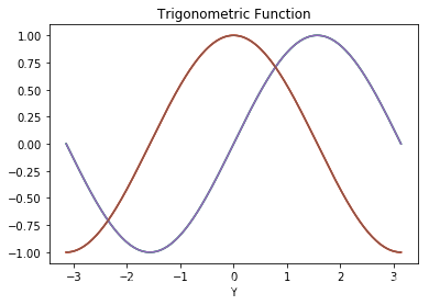
# 简单的三角函数计算
import numpy as np
import pylab as pl
x = np.linspace(-np.pi,np.pi,256)
s = np.sin(x)
c = np.cos(x)
pl.title('Trigonometric Function')
pl.xlabel('X')
pl.xlabel('Y')
pl.plot(x,s)
pl.plot(x,c)
pl.show()
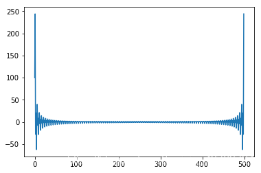
# 一组数据的傅里叶变换
import scipy as sp
import pylab as pl
listA = sp.ones(500)
listA[100:300] = -1
f = sp.fft(listA)
pl.plot(f)
pl.show()
D:\software\Anaconda\anaconda\lib\site-packages\numpy\core\numeric.py:531: ComplexWarning: Casting complex values to real discards the imaginary part
  return array(a, dtype, copy=False, order=order)
# Biopython 功能:将生物信息学文件分析成Python 可利用的数据结构;处理常用的在线生物信息学数据库代码;提供常用生物信息程序的界面
# 序列、字母表和染色体图
from Bio.Seq import Seq
my_seq = Seq("AGTACACTGGT")
print(my_seq.alphabet)
print(my_seq)
07_7 python的人文社科类应用
# 古腾堡项目
from nltk.corpus import Gutenberg
print(gutenberg.fileids)
# 一些简单的计算
from nltk.corpus import Gutenberg
allwords = gutenberg.words('shakespeare-hamlet.txt')
print(len(allwords))
print(len(set(allwords)))
print(all_words.count('Hamlet'))
A = set(allwords)
longwords = [w for w in A if len(w)>12]
print (sorted(longwords))


 858
858

 被折叠的 条评论
为什么被折叠?
被折叠的 条评论
为什么被折叠?
 到【灌水乐园】发言


