CS231n-Lecture Note-06-Training Neural Networks

​
There are three main steps to training a neural network.

1. One-time set-up:

1.1 activation functions

1. About the activation functions, this article has been discussed more deeply.
2. The one we haven’t discussed is maxout
   Maxout applies to the dot product. Compute the function

1.2 preprocessing

1.2.1 Mean subtraction

The most commonly uses in preprocessing. It subtracts the mean across every individual feature in the data. And geomertically, move each dimension’s data around the origin.

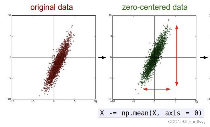
X -= np.mean(X, axis = 0) # substract the mean
# but for a image 
X -= np.mean(X) # no needs to set axis, we need to subtract each channel

1.2.2 Normalization

It normalize the data dimensions and they are appromimately the same scale.
There are two commonly ways to achieve the normalization:

1. Once the data zero-centered processes, then divided the dimensions by mean.

   X /= np.std(X, axis=0)
   

2. Normalize each dimensions, so the max and min along each dimensions is 1 and -1. Only works on inputs are in different scales. But they should be of approximately equal importance to the learning algorithm.
   
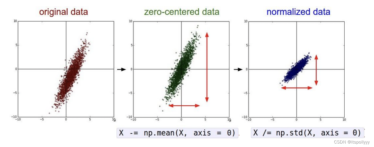
   The double-headed arrow indicate the scale of each dimension. Here is a 2-dimension example. In the third graph the scale of each dimension is same.
   In this lecture which also mentioned PCA/Whitening, but these two are not used with Convolutional Networks. If you wanna deep drag this, please refer to this.

2.weight initialization

2.1 Initialize all weights to 0

If we set all weights to 0, we will get all the same gradients during backpropagation. Update with the same values. Which means there is no source of asymmetry between neurons.

2.2 Small random numbers

The commonly way is initalize the weights with gaussian with zero mean and 1e-2 standard deviation.

W = 0.01 * np.random.randn(Din, Dout)

This is work okay for small networks.
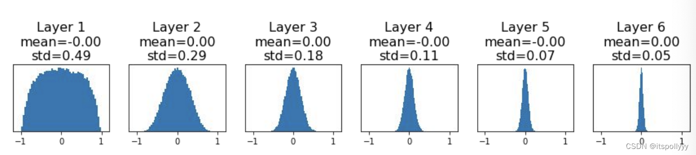
Suppose we have a 6-layer net, hidden size 4096 and the activiation function use tanh.

dims = [4096] * 7
hs = []
x = np.random.randn(16, dims[0])
for Din, Dout in zip(dims[:-1], dims[1:]):
	W = 0.01* np.random.randn(Din, Dout)
	x = np.tanh(x.dot(W))
	hs.append(x)

The activations tend to zero for deeper network layers. There is no learning.

Then we increase the std to 0.05, all activations saturate. The local gradients becomes to zero, no learning as well.

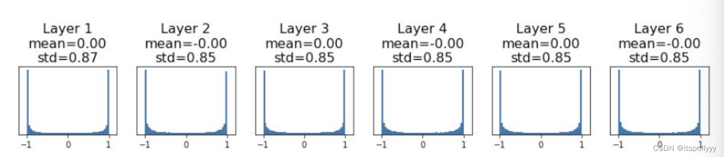
From above, large weight cause the saturate. Another best choose is Xavier.

2.3 Xavier/He initialize

Xavier set std to 1/sqrt(Din)

W = np.random.randn(Din, Dout) / np.sqrt(Din)

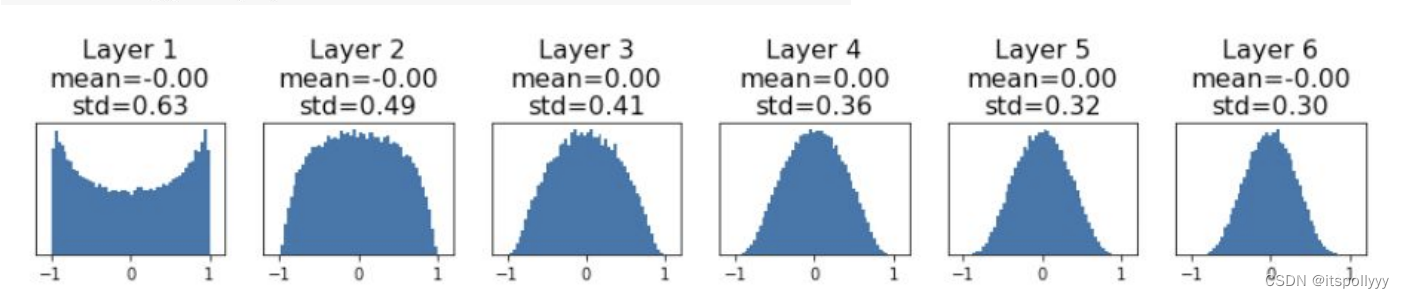
Activations are nicely scaled for all layers. For Conv layers, Din is filter_size^2 * input_channels.
What exactly is Xavier initialization?
Suppose we have n weights, we can initialize weight with Gaussian distrubution.
Suppose we have this equation:
$$y=w_1{x}_1+w_2{x}_2+...+w_n{x}_n+b$$
For each hidden layer, we want each layers’ input and output’s variance not change.
$$va$$