TensorFlow中的神经网络

利用Tensorflow来构建一个基本的神经网络，用于预测手写体数字，采用MNIST数据集。

首先导入Tensorflow 并从 tensorflow.examples.tutorials.mnist加载数据集：

import warnings
warnings.filterwarnings('ignore')
import tensorflow as tf
from tensorflow.examples.tutorials.mnist import input_data
mnist = input_data.read_data_sets("data/mnist/", one_hot=True)

观察数据集中的具体数据：

print("No of images in training set {}".format(mnist.train.images.shape))
print("No of labels in training set {}".format(mnist.train.labels.shape))
print("No of images in test set {}".format(mnist.test.images.shape))
print("No of labels in test set {}".format(mnist.test.labels.shape))

输出为：

No of images in training set (55000, 784)
No of labels in training set (55000, 10)
No of images in test set (10000, 784)
No of labels in test set (10000, 10)

表明训练集中有55000幅图像，且每张图像的大小为784(28x28)。另外，有10种标记，实际上是0~9。同样，在test set中有10000 幅图像。

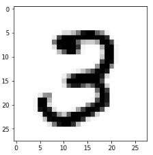
接下来，输出一幅输入图像：

import matplotlib.pyplot as plt
img1 = mnist.train.images[41].reshape(28, 28)
plt.imshow(img1, cmap='Greys')

接下来，构建两层的神经网络。其中包含一个输入层，隐藏层和一个预测手写数字的输出层。

首先定义输入输出占位符。由于数据大小为784。因此，定义输入占位符为：

x = tf.placeholder(tf.float32, [None, 784])

其中，None指定了传递样本的个数(批大小)，这是在运行时动态确定的。

由于输出有10类，因此可定义输出placeholder为：

y = tf.placeholder(tf.float32, [None, 10])

接下来，初始化超参数：

learning_rate = 0.1
batch_size = 100
epochs = 10

然后，定义一个输入层与输出层之间的权重和偏置分别为 w_xh 和 b_h。利用从标准差为0.03的正态分布中随机抽取的值来初始化权重矩阵：

w_ih = tf.Variable(tf.random_normal([784, 300], stddev=0.03), name='w_ih')
b_h = tf.Variable(tf.random_normal([300]), name='b_h')

接着，定义隐层与输出层之间的权重和偏置分别为 w_hy 和 b_y :

w_hy = tf.Variable(tf.random_normal([300, 10], stddev=0.03), name='w_hy')
b_y = tf.Variable(tf.random_normal([10]), name='b_y') 

现在执行前向传播。调用在前向传播中执行的步骤：

z1 = tf.add(tf.matmul(x, w_ih), b_h)
a1 = tf.nn.relu(z1)
z2 = tf.add(tf.matmul(a1, w_hy), b_y)
yhat = tf.nn.softmax(z2)

在此，定义成本函数为交叉熵损失。交叉熵损失也称为对数损失，定义如下：

          $-{\sum }_i{y}_i\log \widehat{y_i}$
式中，$y_i$为实际值，$\widehat{y_i}$ 为预测值

cross_entropy = tf.reduce_mean(-tf.reduce_sum(y * tf.log(yhat), reduction_indices=[1]))

目标是使得成本函数最小化。可通过网络反向传播并执行梯度下降来最小化成本函数。在Tensorflow中，不必手动计算梯度，可利用Tensorflow中的内置梯度下降优化器函数：

optimiser = tf.train.GradientDescentOptimizer(learning_rate=learning_rate).minimize(cross_entropy)

为评估所构建的模型，需要计算精度：

correct_prediction = tf.equal(tf.argmax(y, 1), tf.argmax(yhat, 1))
accuracy = tf.reduce_mean(tf.cast(correct_prediction, tf.float32))

正如已知Tensorflow是通过构建计算图来运行的，因此一旦启动Tensorflow会话，就会只执行现已编写的所有程序。接下来，具体实现。
首先，初始化tensorflow变量：

init_op = tf.global_variables_initializer()

这时，启动tensorflow会话，并开始训练模型：

with tf.Session() as sess:
   sess.run(init_op)
   total_batch = int(len(mnist.train.labels) / batch_size)
    
   for epoch in range(epochs):
        avg_cost = 0
        
        for i in range(total_batch):
            batch_x, batch_y = mnist.train.next_batch(batch_size=batch_size)
            
            _, c = sess.run([optimiser, cross_entropy], 
                         feed_dict={x: batch_x, y: batch_y})
            
            avg_cost += c / total_batch
            
        print("Epoch:", (epoch + 1), "cost =""{:.3f}".format(avg_cost))
        
   print(sess.run(accuracy, feed_dict={x: mnist.test.images, y: mnist.test.labels}))

整理于：7.6 Neural Network Using Tensorflow.ipynb