前向传播和反向传播_神经网络反向传播算法

最新推荐文章于 2025-05-22 21:00:00 发布

原创最新推荐文章于 2025-05-22 21:00:00 发布 · 278 阅读

1 ·

CC 4.0 BY-SA版权

文章标签：

#前向传播和反向传播 #反向传播算法

奇技指南

本文介绍全连接人工神经网络的训练算法——反向传播算法。反向传播算法本质上是梯度下降法。人工神经网络的参数多，梯度计算比较复杂。在人工神经网络模型提出几十年后才有研究者提出了反向传播算法来解决深层参数的训练问题。本文将详细讲解该算法的原理及实现。本篇为机器学习系列文章

一、符号与表示

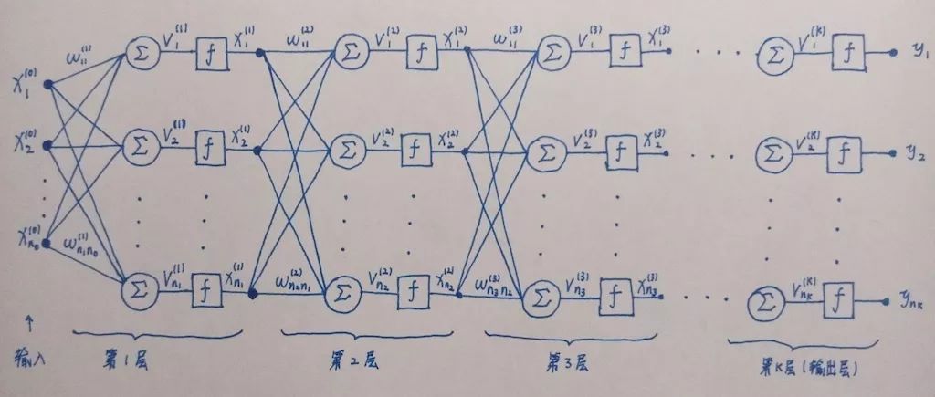
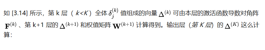
图 1.1 多层全连接神经网络

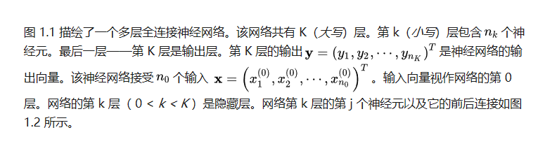
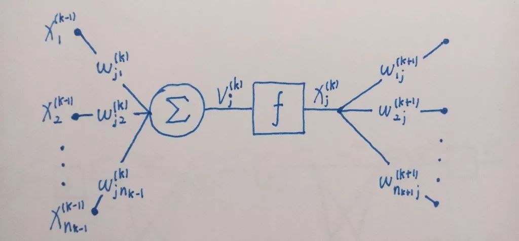
图 1.2 神经元

训练过程

对每一个提交给神经网络的样本用式 [2.3] 对全体权值进行一次更新，直到所有样本的误差值都小于一个预设的阈值，此时训练完成。看到这里或有疑问：不是应该用所有训练样本的误差的模平方的平均值(均方误差)来作 E 么？如果把样本误差的模平方看作一个随机变量，那么所有样本的平均误差模平方是该随机变量的一个无偏估计。而一个样本的误差模平方也是该随机变量的无偏估计，只不过估计得比较粗糙(大数定律)。但是用一次一个样本的误差模平方进行训练可节省计算量，且支持在线学习(样本随来随训练)。

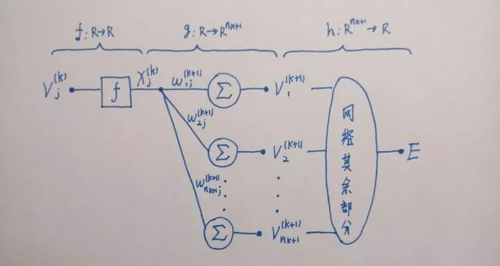
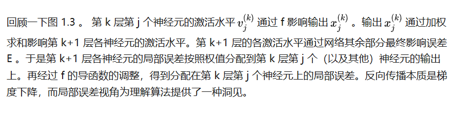
图 1.3 神经网络各个值影响损失函数的方式

反向传播阶段：

权值更新阶段：

将矩阵形式的反向传播与权值更新算法总结如下：

反向传播阶段：

权值更新阶段：

实现

后来笔者写了一个机器学习库。那里的 ANN 实现对本文例程做了改进：

https://link.zhihu.com/?target=https%3A//github.com/zhangjuefei/mentat

本节以 Python 语言实现了一个 mini-batch 随机梯度下降反向传播神经网络，带冲量和学习率衰减功能。代码如下：

import numpy as npclass DNN:    def __init__(self, input_shape, shape, activations, eta=0.1, threshold=1e-5, softmax=False, max_epochs=1000,                 regularization=0.001, minibatch_size=5, momentum=0.9, decay_power=0.5, verbose=False):        if not len(shape) == len(activations):            raise Exception("activations must equal to number od layers.")        self.depth = len(shape)        self.activity_levels = [np.mat([0])] * self.depth        self.outputs = [np.mat(np.mat([0]))] * (self.depth + 1)        self.deltas = [np.mat(np.mat([0]))] * self.depth        self.eta = float(eta)        self.effective_eta = self.eta        self.threshold = float(threshold)        self.max_epochs = int(max_epochs)        self.regularization = float(regularization)        self.is_softmax = bool(softmax)        self.verbose = bool(verbose)        self.minibatch_size = int(minibatch_size)        self.momentum = float(momentum)        self.decay_power = float(decay_power)        self.iterations = 0        self.epochs = 0        self.activations = activations        self.activation_func = []        self.activation_func_diff = []        for f in activations:            if f == "sigmoid":                self.activation_func.append(np.vectorize(self.sigmoid))                self.activation_func_diff.append(np.vectorize(self.sigmoid_diff))            elif f == "identity":                self.activation_func.append(np.vectorize(self.identity))                self.activation_func_diff.append(np.vectorize(self.identity_diff))            elif f == "relu":                self.activation_func.append(np.vectorize(self.relu))                self.activation_func_diff.append(np.vectorize(self.relu_diff))            else:                raise Exception("activation function {:s}".format(f))        self.weights = [np.mat(np.mat([0]))] * self.depth        self.biases = [np.mat(np.mat([0]))] * self.depth        self.acc_weights_delta = [np.mat(np.mat([0]))] * self.depth        self.acc_biases_delta = [np.mat(np.mat([0]))] * self.depth        self.weights[0] = np.mat(np.random.random((shape[0], input_shape)) / 100)        self.biases[0] = np.mat(np.random.random((shape[0], 1)) / 100)        for idx in np.arange(1, len(shape)):            self.weights[idx] = np.mat(np.random.random((shape[idx], shape[idx - 1])) / 100)            self.biases[idx] = np.mat(np.random.random((shape[idx], 1)) / 100)    def compute(self, x):        result = x        for idx in np.arange(0, self.depth):            self.outputs[idx] = result            al = self.weights[idx] * result + self.biases[idx]            self.activity_levels[idx] = al            result = self.activation_func[idx](al)        self.outputs[self.depth] = result        return self.softmax(result) if self.is_softmax else result    def predict(self, x):        return self.compute(np.mat(x).T).T.A    def bp(self, d):        tmp = d.T        for idx in np.arange(0, self.depth)[::-1]:            delta = np.multiply(tmp, self.activation_func_diff[idx](self.activity_levels[idx]).T)            self.deltas[idx] = delta            tmp = delta * self.weights[idx]    def update(self):        self.effective_eta = self.eta / np.power(self.iterations, self.decay_power)        for idx in np.arange(0, self.depth):            # current gradient            weights_grad = -self.deltas[idx].T * self.outputs[idx].T / self.deltas[idx].shape[0] + \                           self.regularization * self.weights[idx]            biases_grad = -np.mean(self.deltas[idx].T, axis=1) + self.regularization * self.biases[idx]            # accumulated delta            self.acc_weights_delta[idx] = self.acc_weights_delta[                                              idx] * self.momentum - self.effective_eta * weights_grad            self.acc_biases_delta[idx] = self.acc_biases_delta[idx] * self.momentum - self.effective_eta * biases_grad            self.weights[idx] = self.weights[idx] + self.acc_weights_delta[idx]            self.biases[idx] = self.biases[idx] + self.acc_biases_delta[idx]    def fit(self, x, y):        x = np.mat(x)        y = np.mat(y)        loss = []        self.iterations = 0        self.epochs = 0        start = 0        train_set_size = x.shape[0]        while True:            end = start + self.minibatch_size            minibatch_x = x[start:end].T            minibatch_y = y[start:end].T            yp = self.compute(minibatch_x)            d = minibatch_y - yp            if self.is_softmax:                loss.append(np.mean(-np.sum(np.multiply(minibatch_y, np.log(yp + 1e-1000)), axis=0)))            else:                loss.append(np.mean(np.sqrt(np.sum(np.power(d, 2), axis=0))))            self.iterations += 1            start = (start + self.minibatch_size) % train_set_size            if self.iterations % train_set_size == 0:                self.epochs += 1                mean_e = np.mean(loss)                loss = []                if self.verbose:                    print("epoch: {:d}. mean loss: {:.6f}. learning rate: {:.8f}".format(self.epochs, mean_e,                                                                                         self.effective_eta))                if self.epochs >= self.max_epochs or mean_e < self.threshold:                    break            self.bp(d)            self.update()    @staticmethod    def sigmoid(x):        return 1.0 / (1.0 + np.power(np.e, min(-x, 1e2)))    @staticmethod    def sigmoid_diff(x):        return np.power(np.e, min(-x, 1e2)) / (1.0 + np.power(np.e, min(-x, 1e2))) ** 2    @staticmethod    def relu(x):        return x if x > 0 else 0.0    @staticmethod    def relu_diff(x):        return 1.0 if x > 0 else 0.0    @staticmethod    def identity(x):        return x    @staticmethod    def identity_diff(x):        return 1.0    @staticmethod    def softmax(x):        x[x > 1e2] = 1e2        ep = np.power(np.e, x)        return ep / np.sum(ep, axis=0)

测试一下神经网络的拟合能力如何。用网络拟合以下三个函数：

对每个函数生成 100 个随机选择的数据点。神经网络的输入为 2 维，输出为 1 维。为每个函数训练 3 个神经网络。这些网络有 1 个隐藏层 1 个输出层，隐藏层神经元数量分别为：3、5 和 8 。隐藏层激活函数是 sigmoid 。输出层的激活函数是恒等函数f(x)=x 。初始学习率 0.4 ，衰减指数 0.2 。冲量惯性 0.6 。迭代 200 个 epoch 。mini batch 样本数为 40 。L2 正则，正则强度 0.0001 。拟合效果见下图：

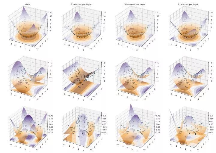
图 4.1 对三种函数进行拟合

测试代码如下：

import numpy as npimport matplotlib.pyplot as pltfrom matplotlib.colors import ListedColormapfrom mentat.classification_model import DNNfrom mpl_toolkits.mplot3d import Axes3Dnp.random.seed(42)hidden_layer_size = [3, 5, 8]  # 隐藏层神经元个数(所有隐藏层都取同样数量神经元)hidden_layers = 1  # 隐藏层数量hidden_layer_activation_func = "sigmoid"  # 隐藏层激活函数learning_rate = 0.4  # 学习率max_epochs = 200  # 训练 epoch 数量regularization_strength = 0.0001  # 正则化强度minibatch_size = 40  # mini batch 样本数momentum = 0.6  # 冲量惯性decay_power = 0.2  # 学习率衰减指数def f1(x):    return (x[:, 0] ** 2 + x[:, 1] ** 2).reshape((len(x), 1))def f2(x):    return (x[:, 0] ** 2 - x[:, 1] ** 2).reshape((len(x), 1))def f3(x):    return (np.cos(1.2 * x[:, 0]) * np.cos(1.2 * x[:, 1])).reshape((len(x), 1))funcs = [f1, f2, f3]X = np.random.uniform(low=-2.0, high=2.0, size=(100, 2))x_min, x_max = X[:, 0].min() - .5, X[:, 0].max() + .5y_min, y_max = X[:, 1].min() - .5, X[:, 1].max() + .5xx, yy = np.meshgrid(np.arange(x_min, x_max, .02), np.arange(y_min, y_max, .02))# 模型names = ["{:d} neurons per layer".format(hs) for hs         in hidden_layer_size]classifiers = [    DNN(input_shape=2, shape=[hs] * hidden_layers + [1],        activations=[hidden_layer_activation_func] * hidden_layers + ["identity"], eta=learning_rate, threshold=0.001,        softmax=False, max_epochs=max_epochs, regularization=regularization_strength, verbose=True,        minibatch_size=minibatch_size, momentum=momentum, decay_power=decay_power) for hs in    hidden_layer_size]figure = plt.figure(figsize=(5 * len(classifiers) + 2, 4 * len(funcs)))cm = plt.cm.PuOrcm_bright = ListedColormap(["#DB9019", "#00343F"])i = 1for cnt, f in enumerate(funcs):    zz = f(np.c_[xx.ravel(), yy.ravel()]).reshape(xx.shape)    z = f(X)    ax = figure.add_subplot(len(funcs), len(classifiers) + 1, i, projection="3d")    if cnt == 0:        ax.set_title("data")    ax.plot_surface(xx, yy, zz, rstride=1, cstride=1, alpha=0.6, cmap=cm)    ax.contourf(xx, yy, zz, zdir='z', offset=zz.min(), alpha=0.6, cmap=cm)    ax.scatter(X[:, 0], X[:, 1], z.ravel(), cmap=cm_bright, edgecolors='k')    ax.set_xlim(xx.min(), xx.max())    ax.set_ylim(yy.min(), yy.max())    ax.set_zlim(zz.min(), zz.max())    i += 1    for name, clf in zip(names, classifiers):        print("model: {:s} training.".format(name))        ax = plt.subplot(len(funcs), len(classifiers) + 1, i)        clf.fit(X, z)        predict = clf.predict(np.c_[xx.ravel(), yy.ravel()]).reshape(xx.shape)        ax = figure.add_subplot(len(funcs), len(classifiers) + 1, i, projection="3d")        if cnt == 0:            ax.set_title(name)        ax.plot_surface(xx, yy, predict, rstride=1, cstride=1, alpha=0.6, cmap=cm)        ax.contourf(xx, yy, predict, zdir='z', offset=zz.min(), alpha=0.6, cmap=cm)        ax.scatter(X[:, 0], X[:, 1], z.ravel(), cmap=cm_bright, edgecolors='k')        ax.set_xlim(xx.min(), xx.max())        ax.set_ylim(yy.min(), yy.max())        ax.set_zlim(zz.min(), zz.max())        i += 1        print("model: {:s} train finished.".format(name))plt.tight_layout()plt.savefig(    "pic/dnn_fitting_{:d}_{:.6f}_{:d}_{:.6f}_{:.3f}_{:3f}.png".format(hidden_layers, learning_rate, max_epochs,                                                                      regularization_strength, momentum, decay_power))

参考书目