scikit-image库-- 基本矩阵估计（十九）

ORB 原理参考

FAST 算法原理

BRIEF 特征描述子

此示例演示了如何使用稀疏ORB特征对应来稳健地估计两个视图之间的极线几何。
基本矩阵涉及一对未校准图像之间的对应点。 矩阵将一个图像中的均匀图像点变换为另一个图像中的极线。
未校准意味着两个摄像机的固有校准（焦距，像素偏斜，主点）未知。 因此，基本矩阵能够实现捕获的场景的投影3D重建。 如果校准已知，则估计基本矩阵使得能够对捕获的场景进行度量3D重建。

import numpy as np
from skimage import data
from skimage.color import rgb2gray
from skimage.feature import match_descriptors, ORB, plot_matches
from skimage.measure import ransac
from skimage.transform import FundamentalMatrixTransform
import matplotlib.pyplot as plt
%matplotlib inline

np.random.seed(0)

img_left, img_right, groundtruth_disp = data.stereo_motorcycle()
img_left, img_right = map(rgb2gray, (img_left, img_right))

# Find sparse feature correspondences between left and right image.

descriptor_extractor = ORB()

descriptor_extractor.detect_and_extract(img_left)
keypoints_left = descriptor_extractor.keypoints #关键点左图
descriptors_left = descriptor_extractor.descriptors

descriptor_extractor.detect_and_extract(img_right)
keypoints_right = descriptor_extractor.keypoints#关键点位置右图 500X2
descriptors_right = descriptor_extractor.descriptors #每个关键点1X256维  总共500X256

matches = match_descriptors(descriptors_left, descriptors_right,
                            cross_check=True)  #相匹配关键点的返回坐标值 【1~500】，有223个匹配，(223, 2)

# Estimate the epipolar geometry between the left and right image.

model, inliers = ransac((keypoints_left[matches[:, 0]], #model为模型参数 ，inliners 相匹配的坐标值 163X1
                         keypoints_right[matches[:, 1]]),
                        FundamentalMatrixTransform, min_samples=8,
                        residual_threshold=1, max_trials=5000)
#第一和第二组描述符中相应匹配的索引，其中匹配[：，0]表示第一组中的索引，并匹配第二组描述符中的索引[：，1]。model：具有最大共识集的最佳模型。inliers：数组分类为True的内部的布尔掩码


inlier_keypoints_left = keypoints_left[matches[inliers, 0]]
inlier_keypoints_right = keypoints_right[matches[inliers, 1]]

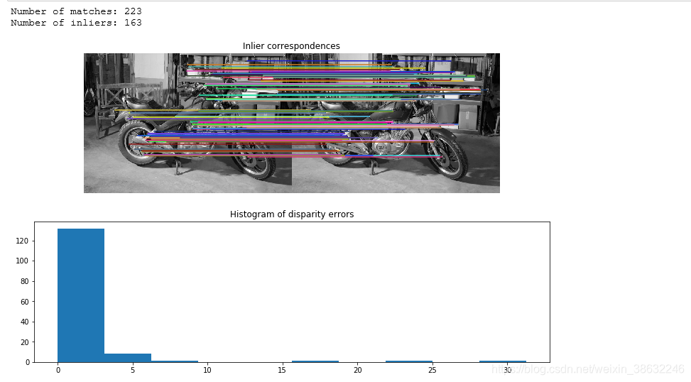
print("Number of matches:", matches.shape[0])
print("Number of inliers:", inliers.sum())

# Compare estimated sparse disparities to the dense ground-truth disparities.

disp = inlier_keypoints_left[:, 1] - inlier_keypoints_right[:, 1]
disp_coords = np.round(inlier_keypoints_left).astype(np.int64) #浮点转整形
disp_idxs = np.ravel_multi_index(disp_coords.T, groundtruth_disp.shape)
disp_error = np.abs(groundtruth_disp.ravel()[disp_idxs] - disp)
disp_error = disp_error[np.isfinite(disp_error)]

# Visualize the results.

fig, ax = plt.subplots(nrows=2, ncols=1,figsize=(13,8))

plt.gray()

plot_matches(ax[0], img_left, img_right, keypoints_left, keypoints_right,
             matches[inliers], only_matches=True)
ax[0].axis("off")
ax[0].set_title("Inlier correspondences")

ax[1].hist(disp_error)
ax[1].set_title("Histogram of disparity errors")

plt.show()