# coding:utf-8
import numpy as np
from sklearn import linear_model, datasets
import matplotlib.pyplot as plt
from scipy.stats import norm
from scipy import fft
from scipy.io import wavfile
n = 40
# hstack数据拼接
# rvs是Random Variates随机变量的意思
# 在模拟X的时候使用了两个正态分布,分别制定各自的均值,方差,生成40个点
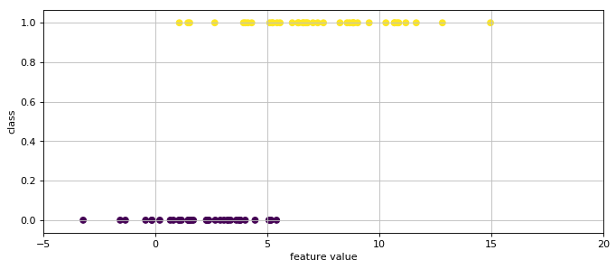
X = np.hstack((norm.rvs(loc=2, size=n, scale=2), norm.rvs(loc=8, size=n, scale=3)))
# zeros使得数据点生成40个0,ones使得数据点生成40个1
y = np.hstack((np.zeros(n), np.ones(n)))
# 创建一个 10 * 4 点(point)的图,并设置分辨率为 80
plt.figure(figsize=(10, 4), dpi=80)
# 设置横轴的上下限
plt.xlim((-5, 20))
# scatter散点图
plt.scatter(X, y, c=y)
plt.xlabel("feature value")
plt.ylabel("class")
plt.grid(True, linestyle='-', color='0.75')
plt.savefig("C:/Users/zhen/Desktop/logistic_classify.png", bbox_inches="tight")
# linspace是在-5到15的区间内找10个数
xs = np.linspace(-5, 15, 10)
# ---linear regression----------
from sklearn.linear_model import LinearRegression
clf = LinearRegression()
# reshape重新把array变成了80行1列二维数组,符合机器学习多维线性回归格式
clf.fit(X.reshape(n * 2, 1), y)
def lin_model(clf, X):
return clf.intercept_ + clf.coef_ * X
# --logistic regression--------
from sklearn.linear_model import LogisticRegression
logclf = LogisticRegression()
# reshape重新把array变成了80行1列二维数组,符合机器学习多维线性回归格式
logclf.fit(X.reshape(n * 2, 1), y)
def lr_model(clf, X):
return 1.0 / (1.0 + np.exp(-(clf.intercept_ + clf.coef_ * X)))
# ----plot---------------------------
plt.figure(figsize=(10, 5))
# 创建一个一行两列子图的图像中第一个图
plt.subplot(1, 2, 1)
plt.scatter(X, y, c=y)
plt.plot(X, lin_model(clf, X), "o", color="orange")
plt.plot(xs, lin_model(clf, xs), "-", color="green")
plt.xlabel("feature value")
plt.ylabel("class")
plt.title("linear fit")
plt.grid(True, linestyle='-', color='0.75')
# 创建一个一行两列子图的图像中第二个图
plt.subplot(1, 2, 2)
plt.scatter(X, y, c=y)
plt.plot(X, lr_model(logclf, X).ravel(), "o", color="c")
plt.plot(xs, lr_model(logclf, xs).ravel(), "-", color="green")
plt.xlabel("feature value")
plt.ylabel("class")
plt.title("logistic fit")
plt.grid(True, linestyle='-', color='0.75')
plt.tight_layout(pad=0.4, w_pad=0, h_pad=1.0)
plt.savefig("C:/Users/zhen/Desktop/logistic_classify2.png", bbox_inches="tight")
结果:
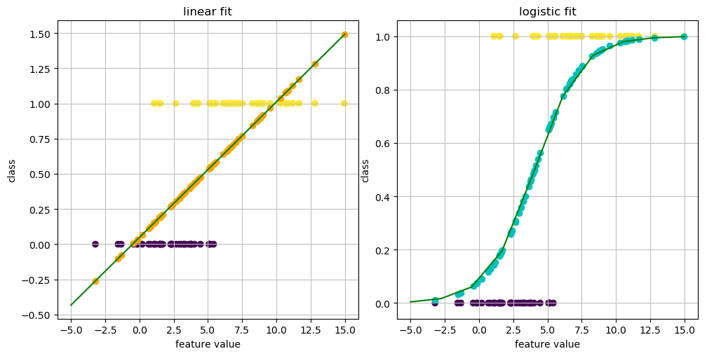


 本文通过生成模拟数据集并使用线性和逻辑回归两种方法进行拟合,展示了这两种回归方法在分类任务上的不同表现。文章详细介绍了如何用Python实现这两种模型,并通过图表直观地比较了它们的预测结果。


 被折叠的 条评论
为什么被折叠?
被折叠的 条评论
为什么被折叠?
 到【灌水乐园】发言


