Introduction to evaluating binary classifiers

2019独角兽企业重金招聘Python工程师标准>>>

1: Introduction To The Data

In the previous mission, we learned about classification, logistic regression, and how to use scikit-learn to fit a logistic regression model to a dataset on graduate school admissions. We'll continue to work with the dataset, which contains data on 644 applications with the following columns:

• gre - applicant's store on the Graduate Record Exam, a generalized test for prospective graduate students.
  • Score ranges from 200 to 800.
• gpa - college grade point average.
  • Continuous between 0.0 and 4.0.
• admit - binary value
  • Binary value, 0 or 1, where 1 means the applicant was admitted to the program and 0 means the applicant was rejected.

Here's a preview of the dataset:

 

admit	gpa	gre
0	3.177277	594.102992
0	3.412655	631.528607
0	2.728097	553.714399
0	3.093559	551.089985
0	3.141923	537.184894

 

To start, let's use the logistic regression model we fit in the last mission to predict the class labels for each observation in the dataset and add these labels to the Dataframe in a separate column.

Instructions

• Use the LogisticRegression method predict to return the label for each observation in the dataset, admissions. Assign the returned list to labels.
• Add a new column to theadmissions Dataframe namedpredicted_label that contains the values from labels.
• Use the Series methodvalue_counts and the printfunction to display the distribution of the values in thelabel column.
• Use the Dataframe method headand the print function to display the first 5 rows inadmissions.

import pandas as pd
import matplotlib.pyplot as plt
%matplotlib inline
from sklearn.linear_model import LogisticRegression

admissions = pd.read_csv("admissions.csv")

model = LogisticRegression()
model.fit(admissions[["gpa"]], admissions["admit"])
labels=model.predict(admissions[["gpa"]])
admissions["predicted_label"]=labels
print(admissions["predicted_label"].value_counts())
print(admissions.head(5))

 

2: Accuracy

The admissions Dataframe now contains the predicted value for that row, in the predicted_label column, and the actual value for that row, in the admit column. This format makes it easier for us to calculate how effective the model was on the training data. The simplest way to determine the effectiveness of a classification model is prediction accuracy. Accuracy helps us answer the question:

• What fraction of the predictions were correct (actual label matched predicted label)?

Prediction accuracy boils down to the number of labels that were correctly predicted divided by the total number of observations:

Accuracy=# of Correctly Predicted# of ObservationsAccuracy=# of Correctly Predicted# of Observations

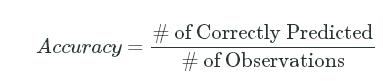
In logistic regression, recall that the model's output is a probability between 0 and 1. To decide who gets admitted, we set a threshold and accept all of the students where their computed probability exceeds that threshold. This threshold is called the discrimination thresholdand scikit-learn sets it to 0.5 by default when predicting labels. If the predicted probability is greater than 0.5, the label for that observation is 1. If it is instead less than 0.5, the label for that observation is 0.

An accuracy of 1.0 means that the model predicted 100% of admissions correctly for the given discrimination threshold. An accuracy of 0.2means that the model predicted 20% of the admissions correctly. Let's calculate the accuracy for the predictions the logistic regression model made.

Instructions

• Rename the admit column from the admissions Dataframe toactual_label so it's more clear which column contains the predicted labels (predicted_label) and which column contains the actual labels (actual_label).
• Compare the predicted_labelcolumn with the actual_labelcolumn.
  • Use a double equals sign (==) to compare the 2 Series objects and assign the resulting Series object to matches.
• Use conditional filtering to filteradmissions to just the rows where matches is True. Assign the resulting Dataframe tocorrect_predictions.
  • Display the first 5 rows incorrect_predictions to make sure the values in thepredicted_label andactual_label columns are equal.
• Calculate the accuracy and assign the resulting float value toaccuracy.
  • Display accuracy using the print function.

labels = model.predict(admissions[["gpa"]])
admissions["predicted_label"] = labels
admissions["actual_label"] = admissions["admit"]
matches = admissions["predicted_label"] == admissions["actual_label"]
correct_predictions = admissions[matches]
print(correct_predictions.head())
accuracy = len(correct_predictions) / len(admissions)
print(accuracy)

3: Binary Classification Outcomes

It looks like the raw accuracy is around 64.6% which is better than randomly guessing the label (which would result in around a 50%accuracy). Calculating the accuracy of a model on the dataset used for training is a useful initial step just to make sure the model at least beats randomly assigning a label for each observation. However, prediction accuracy doesn't tell us much more.

The accuracy doesn't tell us how the model performs on data it wasn't trained on. A model that returns a 100% accuracy when evaluated on it's training set doesn't tell us how well the model works on data it's never seen before (and wasn't trained on). Accuracy also doesn't help us discriminate between the different types of outcomes a binary classification model can make. In a later mission, we'll learn how to evaluate a model's effectiveness on new, unseen data. In this mission, we'll focus on the principles of evaluating binary classification models by testing our model's effectiveness on the training data.

To start, let's discuss the 4 different outcomes of a binary classification model:

 

Prediction	Observation
	Admitted (1)	Rejected (0)
Admitted (1)	True Positive (TP)	False Positive (FP)
Rejected (0)	False Negative (FN)	True Negative (TN)

 

By segmenting a model's predictions into these different outcome categories, we can start to think about other measures of effectiveness that give us more granularity than simple accuracy.

We can define these outcomes as:

• True Postive - The model correctly predicted that the student would be admitted.

  • Said another way, the model predicted that the label would be Positive, and that ended up being True.
  • In our case, Positive refers to being admitted and maps to the label 1 in the dataset.
  • For this dataset, a true positive is whenever predicted_label is 1 and actual_label is 1.

• True Negative - The model correctly predicted that the student would be rejected.

  • Said another way, the model predicted that the label would be Negative, and that ended up being True.
  • In our case, Negative refers to being rejected and maps to the label 0 in the dataset.
  • For this dataset, a true negative is whenever predicted_label is 0 and actual_label is 0.

• False Positive - The model incorrectly predicted that the student would be admitted even though the student was actually rejected.

  • Said another way, the model predicted that the label would be Positive, but that was False (the actual label was True).
  • For this dataset, a false positive is whenever predicted_label is 1 but the actual_label is 0.

• False Negative - The model incorrectly predicted that the student would be rejected even though the student was actually admitted.

  • Said another way, the model predicted that the would be Negative, but that was False (the actual value was True).
  • For this dataset, a false negative is whenever predicted_label is 0 but the actual_label is 1.

Let's calculate the number of observations that fall into some of these outcome categories.

Instructions

• Extract all of the rows wherepredicted_label andactual_label both equal 1. Then, calculate the number of true positives and assign totrue_positives.

• Extract all of the rows wherepredicted_label andactual_label both equal 0. Then, calculate the number of true negatives and assign totrue_negatives.

• Use the print function to display both true_positivesand true_negatives.

true_positives=len(admissions[(admissions["predicted_label"]==1)&(admissions["actual_label"]==1)])
true_negatives=len(admissions[(admissions["predicted_label"]==0)&(admissions["actual_label"]==0)])
print(true_positives)
print(true_negatives)
False_positives=len(admissions[(admissions["predicted_label"]==1)&(admissions["actual_label"]==0)])
False_negatives=len(admissions[(admissions["predicted_label"]==0)&(admissions["actual_label"]==1)])
print(False_positives)
print(False_negatives)
print(admissions.shape[0])

4: Sensitivity

Let's now look at a few measures that are much more insightful than simple accuracy. Let's start with sensitivity:

• Sensitivity or True Postive Rate - The proportion of applicants that were correctly admitted:

TPR=True PositivesTrue Positives+False NegativesTPR=True PositivesTrue Positives+False Negatives

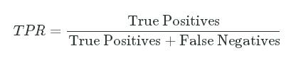
Of all of the students that should have been admitted (True Positives + False Negatives), what fraction did the model correctly admit (True Positives)? More generally, this measure helps us answer the question:

• How effective is this model at identifying positive outcomes?

In our case, the positive outcome (label of 1) is admitting a student. If the True Positive Rate is low, it means that the model isn't effective at catching positive cases. For certain problems, high sensitivity is incredibly important. If we're building a model to predict which patients have cancer, every patient that is missed by the model could mean a loss of life. We want a highly sensitive model that is able to "catch" all of the positive cases (in this case, the positive case is a patient with cancer).

Let's calculate the sensitivity for the model we're working with.

Instructions

• Calculate the number of false negatives (where the model predicted rejected but the student was actually admitted) and assign to false_negatives.
• Calculate the sensitivity and assign the computed value tosensitivity.

# From the previous screen
true_positive_filter = (admissions["predicted_label"] == 1) & (admissions["actual_label"] == 1)
true_positives = len(admissions[true_positive_filter])
false_negatives=len(admissions[(admissions["predicted_label"]==0)&(admissions["actual_label"]==1)])
sensitivity=true_positives/(false_negatives+true_positives)
print(sensitivity)

 

5: Specificity

Looks like the sensitivity of the model is around 12.7% and only about 1 in 8 students that should have been admitted were actually admitted. In the context of predicting student admissions, this probably isn't too bad of a thing. Graduate schools can only admit a select number of students into their programs and by definition they end up rejecting many qualified students that would have succeeded.

In the healthcare context, however, low sensitivity could mean a severe loss of life. If a classification model is only catching 12.7% of positive cases for an illness, then around 7 of 8 people are going undiagnosed (being classified as false negatives). Hopefully you're beginning to acquire a sense for the tradeoffs predictive models make and the importance of understanding the various measures.

Let's now learn about specificity:

• Specificity or True Negative Rate - The proportion of applicants that were correctly rejected:

TNR=True NegativesFalse Positives+True NegativesTNR=True NegativesFalse Positives+True Negatives

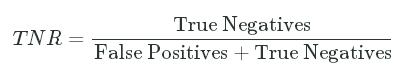
This helps us answer the question:

• How effective is this model at identifying negative outcomes?

In our case, the specificity tells us the proportion of applicants who should be rejected (actual_label equal to 0, which consists of False Positives + True Negatives) that were correctly rejected (just True Negatives). A high specificity means that the model is really good at predicting which applicants should be rejected.

Let's calculate the specificity of our model.

Instructions

• Calculate the number of false positives (where the model predicted admitted but the student was actually rejected) and assign to false_positives.
• Calculate the specificity and assign the computed value tospecificity.

# From previous screens
true_positive_filter = (admissions["predicted_label"] == 1) & (admissions["actual_label"] == 1)
true_positives = len(admissions[true_positive_filter])
false_negative_filter = (admissions["predicted_label"] == 0) & (admissions["actual_label"] == 1)
false_negatives = len(admissions[false_negative_filter])
true_negative_filter = (admissions["predicted_label"] == 0) & (admissions["actual_label"] == 0)
true_negatives = len(admissions[true_negative_filter])
false_positives=len(admissions[(admissions["predicted_label"] == 1) & (admissions["actual_label"] == 0)])
specificity=true_negatives/(true_negatives+false_positives)
print(specificity)

6: Next Steps

It looks like the specificity of the model is 96.25%. This means that the model is really good at knowing which applicants to reject. Since around only 7% of applicants were accepted that applied, it's important that the model reject people correctly who wouldn't have otherwise been accepted.

In this mission, we learned about some of the different ways of evaluating how well a binary classification model performs. The different measures we learned about have very similar names and it's easy to confuse them. Don't fret! The important takeaway is the ability to frame the question you want to answer and working backwards from that to formulate the correct calculation.

If you want to know how well a binary classification model is at catching positive cases, you should have the intuition to divide the correctly predicted positive cases by all actually positive cases. There are 2 outcomes associated with an admitted student (positive case), a false negative and a true positive. Therefore, by dividing the number of true positives by the sum of false negatives and true positives, you'll have the proportion corresponding to the model's effectiveness of identifying positive cases. While this proportion is referred to as the sensitivity, the word itself is secondary to the concept and being able to work backwards to the formula!

These measures are just a starting point, however, and aren't super useful by themselves. In the next mission, we'll dive into cross-validation, where we'll evaluate our model's accuracy on new data that it wasn't trained on. In addition, we'll explore how varying the discrimination threshold affects the measures we learned about in this mission. These important techniques help us gain a much more complete understanding of a classification model's performance.

 

 

 

 

 

 

转载于:https://my.oschina.net/Bettyty/blog/751331