%% 修正后的机械臂轨迹规划系统 (维度问题修复)
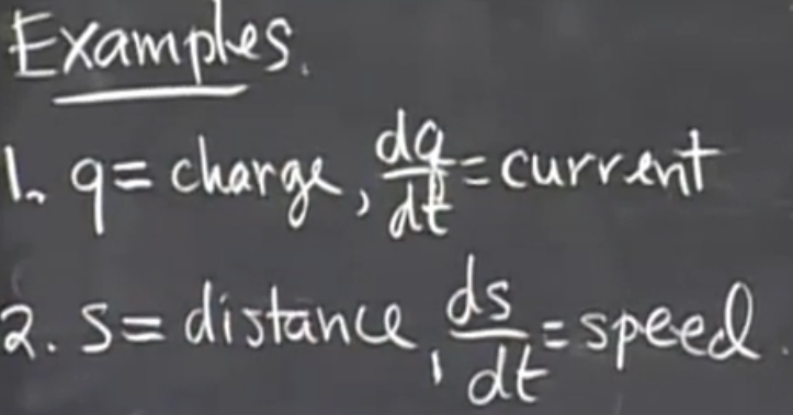
clear; clc; close all;
% ===========================================
% 主程序 (修正维度问题)
% ===========================================
% 机械臂参数 (Modified D-H)
a = [0, 0, 500, 500, 0, 0]; % 连杆长度(mm)
alpha = [0, -pi/2, 0, -pi/2, pi/2, -pi/2]; % 连杆扭角(rad)
d = [400, 0, 0, 0, 0, 100]; % 连杆偏移(mm)
joint_limits = [
-pi, pi; % 关节1
-pi/2, pi/2; % 关节2
-pi/2, pi/2; % 关节3
-pi, pi; % 关节4
0, pi; % 关节5
-pi, pi % 关节6
];
% 选择工作空间中的两点
P_start = [600; 200; 500];
P_goal = [300; -300; 600];
R = [1 0 0; 0 -1 0; 0 0 -1]; % 旋转矩阵(末端垂直向下)
T_start = [R, P_start; 0 0 0 1];
T_goal = [R, P_goal; 0 0 0 1];
% 自定义逆运动学求解
q_start_sols = inverse_kinematics(T_start, a, alpha, d, joint_limits);
q_goal_sols = inverse_kinematics(T_goal, a, alpha, d, joint_limits);
% 使用改进的选择函数
current_position = [0, 0, 0, 0, pi/2, 0]; % 假设初始位置
if isempty(q_start_sols)
error('初始位置逆运动学无解!');
else
q_start = select_solution(q_start_sols, current_position, joint_limits);
end
if isempty(q_goal_sols)
error('目标位置逆运动学无解!');
else
q_goal = select_solution(q_goal_sols, q_start, joint_limits);
end
% 显示选择结果
fprintf('选择的初始关节角度: [%.2f°, %.2f°, %.2f°, %.2f°, %.2f°, %.2f°]\n', rad2deg(q_start));
fprintf('选择的终止关节角度: [%.2f°, %.2f°, %.2f°, %.极f°, %.2f°, %.2f°]\n', rad2deg(q_goal));
% ===========================================
% PTP轨迹规划 (五次多项式插值)
% ===========================================
t_total = 5; % 总时间5秒
t = linspace(0, t_total, 500); % 时间向量
q_traj = zeros(length(t), 6); % 轨迹存储
% 对每个关节进行轨迹规划
for i = 1:6
% 边界条件设置
A = [1, 0, 0, 0, 极, 0;
0, 1, 0, 0, 0, 0;
0, 0, 2, 0, 0, 0;
1, t_total, t_total^2, t_total^3, t_total^4, t_total^5;
0, 1, 2*t_total, 3*t_total^2, 4*t_total^3, 5*t_total^4;
0, 0, 2, 6*t_total, 12*t_total^2, 20*t_total^3];
b = [q_start(i); 0; 0; q_goal(i); 0; 0];
coeff = A \ b; % 求解多项式系数
% 计算轨迹
q_traj(:, i) = polyval(flip(coeff'), t);
end
% ===========================================
% 绘制关节轨迹曲线
% ===========================================
figure('Name', '关节轨迹曲线', 'Color', 'white', 'Position', [100, 100, 1200, 800]);
joint_names = {'关节1', '关节2', '关节3', '关节4', '关节5', '关节6'};
for i = 1:6
subplot(2, 3, i);
plot(t, rad2deg(q_traj(:, i)), 'LineWidth', 2);
hold on;
% 标记起点和终点
plot(0, rad2deg(q_start(i)), 'ro', 'MarkerSize', 8, 'MarkerFaceColor', 'r');
plot(t_total, rad2deg(q_goal(i)), 'go', 'MarkerSize', 8, 'MarkerFaceColor', 'g');
grid on;
title(sprintf('%s 轨迹', joint_names{i}));
xlabel('时间 (s)');
ylabel('关节角度 (deg)');
legend('轨迹', '起点', '终点', 'Location', 'best');
% 添加关节限制线
yline(rad2deg(joint_limits(i, 1)), 'r--', 'LineWidth', 1.5);
yline(rad2deg(joint_limits(i, 2)), 'r--', 'LineWidth', 1.5);
end
sgtitle(sprintf('机械臂PTP轨迹控制 (%.1fs)', t_total));
% ===========================================
% 修正后的函数定义 (修复维度问题)
% ===========================================
% 改进的逆解选择函数
function selected = select_solution(solutions, reference, joint_limits)
if isempty(solutions)
error('逆运动学无解!');
end
% 确保解决方案是N×6矩阵
if size(solutions, 2) == 1 && size(solutions, 1) == 6
solutions = solutions'; % 转置为行向量
end
if size(solutions, 2) ~= 6
error('逆解矩阵维度错误,应为N×6矩阵,实际为%d×%d', ...
size(solutions, 1), size(solutions, 2));
end
% 筛选有效解
valid_solutions = solutions;
valid_mask = true(size(valid_solutions, 1), 1);
for i = 1:size(valid_solutions, 1)
for j = 1:6
angle = valid_solutions(i, j);
% 角度周期性处理
while angle < joint_limits(j, 1)
angle = angle + 2*pi;
end
while angle > joint_limits(j, 2)
angle = angle - 2*pi;
end
if angle < joint_limits(j, 1) || angle > joint_limits(j, 2)
valid_mask(i) = false;
break;
end
end
end
valid_solutions = valid_solutions(valid_mask, :);
% 无有效解处理
if isempty(valid_solutions)
warning('所有逆解均超出关节限位,使用最佳近似解');
valid_solutions = solutions;
end
% 选择最优解
displacements = zeros(size(valid_solutions, 1), 1);
for i = 1:size(valid_solutions, 1)
diff = abs(valid_solutions(i, :) - reference);
periodic_diff = min(diff, 2*pi - diff); % 周期性差异
displacements(i) = norm(periodic_diff);
end
% 避免奇异构型
singularity_penalty = ones(size(valid_solutions, 1), 1);
for i = 1:size(valid极olutions, 1)
if abs(valid_solutions(i, 5)) < deg2rad(5)
singularity_penalty(i) = 10; % 增加惩罚
end
end
[~, idx] = min(displacements .* singularity_penalty);
selected = valid_solutions(idx, :);
end
% 修正的逆运动学函数
function solutions = inverse_kinematics(T, a, alpha, d, joint_limits)
P = T(1:3, 4);
x = P(1); y = P(2); z = P(3);
R = T(1:3, 1:3);
solutions = [];
% 关节1求解选项
theta1_options = [atan2(y, x), atan2(y, x) + pi, atan2(y, x) - pi];
% 关节3参数计算
c3 = (x^2 + y^2 + (z - d(1))^2 - a(2)^2 - a(3)^2 - d(4)^2) / (2 * a(2) * a(3));
% 可达性检查
if abs(c3) > 1
sol = numerical_ik(T, a, alpha, d, joint_limits);
solutions = sol;
return;
end
s3_options = [sqrt(1 - c3^2), -sqrt(1 - c3^2)];
for theta1 = theta1_options
for s3 = s3_options
theta3 = atan2(s3, c3);
% 关节2求解
A = a(2) + a(3)*c3;
B = a(3)*s3;
k1 = A*cos(theta1) + B*sin(theta1);
k2 = A*sin(theta1) - B*cos(theta1);
k3 = z - d(1);
denom = k1^2 + k2^2;
if abs(denom) < 1e-6
continue;
end
r = sqrt(k1^2 + k2^2);
sin_phi = k1 / r;
cos_phi = k2 / r;
sin_theta2 = (k3*cos_phi + sqrt(r^2 - k3^2)*sin_phi) / r;
cos_theta2 = (k1 - B*sin_theta2) / A;
theta2 = atan2(sin_theta2, cos_theta2);
% 正向运动学验证
T01 = dh_transform(a(1), alpha(1), d(1), theta1);
T12 = dh_transform(a(2), alpha(2), d(2), theta2);
T23 = dh_transform(a(3), alpha(3), d(3), theta3);
T03 = T01 * T12 * T23;
R03 = T03(1:3, 1:3);
R36 = R03' * R;
% ZYZ欧拉角分解
[theta4, theta5, theta6] = zyz_euler(R36);
% 保存解
for k = 1:2
sol = [theta1, theta2, theta3, theta4(k), theta5(k), theta6(k)];
solutions = [solutions; sol];
end
end
end
% 数值优化备用
if isempty(solutions)
sol = numerical_ik(T, a, alpha, d, joint_limits);
solutions = [solutions; sol];
end
end
% 修正的数值逆运动学函数 (修复维度问题)
function solution = numerical_ik(T, a, alpha, d, joint_limits)
% 关键修正:确保joint_limits是6×2矩阵
[m, n] = size(joint_limits);
if m == 2 && n == 6
% 转置为6×2
joint_limits = joint_limits';
warning('numerical_ik: joint_limits transposed from 2x6 to 6x2');
elseif m ~= 6 || n ~= 2
error('numerical_ik: joint_limits must be 6x2, but got %dx%d', m, n);
end
options = optimoptions('fmincon', 'Display', 'notify', ...
'Algorithm', 'sqp', 'MaxIterations', 500);
% 关键修正:确保初始猜测是6×1向量
q0 = mean(joint_limits, 2); % 按行平均,得到6×1向量
q0 = q0(:); % 确保列向量 (6×1)
% 目标函数:位姿误差
objective = @(q) norm(forward_kinematics(q, a, alpha, d) - T, 'fro');
% 确保边界是6×1向量
lb = joint_limits(:, 1);
lb = lb(:); % 确保列向量
ub = joint_limits(:, 2);
ub = ub(:); % 确保列向量
% 验证维度匹配
if length(q0) ~= 6
error('q0维度错误: %d,应为6', length(q0));
end
if length(lb) ~= 6
error('lb维度错误: %d,应为6', length(lb));
end
if length(ub) ~= 6
error('ub维度错误: %d,应为6', length(ub));
end
[q_opt, ~, exitflag] = fmincon(objective, q0, [], [], [], [], ...
lb, ub, [], options);
if exitflag > 0
solution = q_opt'; % 转置为行向量 (1×6)
else
% 尝试随机初始值
warning('数值优化失败,尝试随机初始值');
for trial = 1:5
q0_rand = lb + (ub - lb).*rand(6,1); % 确保6×1向量
[q_opt, ~, exitflag] = fmincon(objective, q0_rand, [], [], [], [], ...
lb, ub, [], options);
if exitflag > 0
solution = q_opt';
return;
end
end
error('数值优化失败,请检查目标位姿是否可达');
end
end
% D-H变换函数
function T = dh_transform(a, alpha, d, theta)
ct = cos(theta);
st = sin(theta);
ca = cos(alpha);
sa = sin(alpha);
T = [ct, -st*ca, st*sa, a*ct;
st, ct*ca, -ct*sa, a*st;
0, sa, ca, d;
0, 0, 0, 1];
end
% 正向运动学函数
function T = forward_kinematics(q, a, alpha, d)
T = eye(4);
for i = 1:length(q)
T = T * dh_transform(a(i), alpha(i), d(i), q(i));
end
end
% ZYZ欧拉角分解
function [theta4, theta5, theta6] = zyz_euler(R)
if abs(R(3,3)) > 0.9999
theta5 = 0;
theta4 = 0;
theta6 = atan2(R(2,1), R(1,1));
theta4_alt = theta4;
theta6_alt = theta6;
else
theta5 = atan2(sqrt(R(1,3)^2 + R(2,3)^2), R(3,3));
theta4 = atan2(R(2,3)/sin(theta5), R(1,3)/sin(theta5));
theta6 = atan2(R(3,2)/sin(theta5), -R(3,1)/sin(theta5));
theta5_alt = -theta5;
theta4_alt = atan2(R(2,3)/sin(theta5_alt), R(1,3)/sin(theta5_alt));
theta6_alt = atan2(R(3,2)/sin(theta5_alt), -R(3,1)/sin(theta5_alt));
end
theta4 = [theta4, theta4_alt];
theta5 = [theta5, theta5_alt];
theta6 = [theta6, theta6_alt];
end
% 辅助函数
function deg = rad2deg(rad)
deg = rad * 180 / pi;
end
function rad = deg2rad(deg)
rad = deg * pi / 180;
end
(改错)


 本文首先从几何角度解释导数,随后介绍了导数作为变化率的概念,并通过具体例子阐述了平均变化率与瞬时变化率的区别。此外,还讨论了函数的连续性和不同类型的间断点。
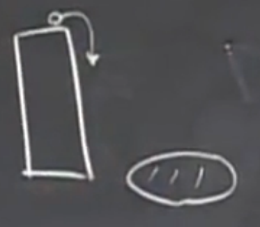 假设一个人站在教学楼上面向一片草地上扔一个南瓜(Pumpkin drop 南瓜坠游戏),楼的高度为80m , 由此可得高度随时间的变化公式为 h = 80 - 5*t2 所以当 t = 0 则 h = 80。当t = 4 则 h =0 所以Ave speed : Δh/Δt = (0-8)/(4-0) 这个是平均速度 下面我们讲一下瞬时速度。 dh/dt = 我们可以根据上一节我们得到的公式 (xn )” = n*xn-1 来对这个公式进行求导。dh/dt = 0 - 10*t . 所以当t = 0 则 h“ = 0,当t = 4 则h” =40 。 所以当落地的时候速度为40。这是平均速度的二倍。
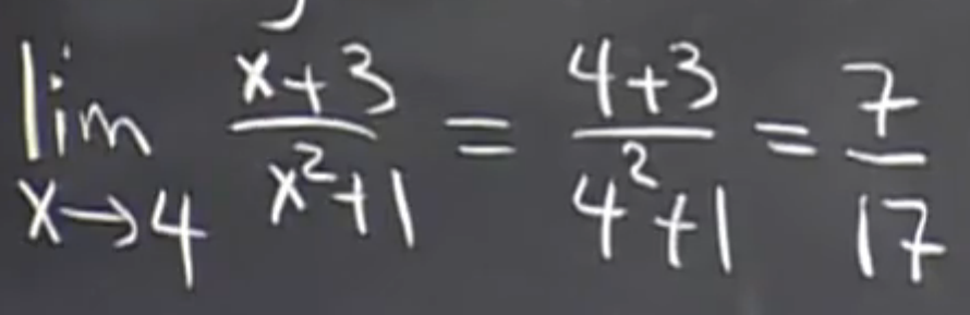 十分简单,这个是简单极限。
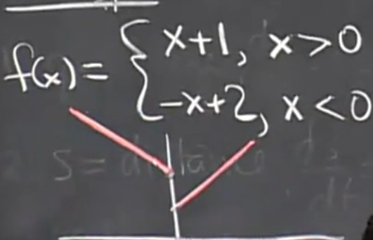 (图中和y轴相交的两点需要用一个园扩起来,表示不包含这一点。)对这一题进行求左右极限得 :
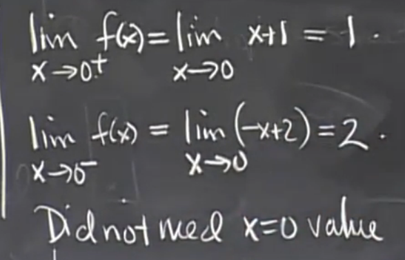 求极限不需要知道 x = 0的值 。
 。
。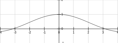 通过图形可得
 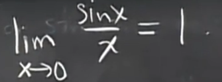 当 x = 0 的时候 该点是没有对应的值得 。
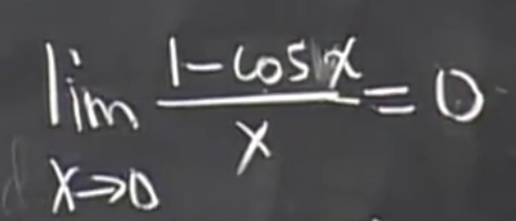 这两个都是 “ 可去间断点 ” 。
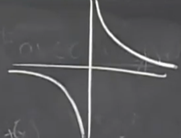 这里要分左右连续。我们可以得到他的左右极限为:
  如果我们部分左右极限直接让他为正无穷或者负无穷的化,这是十分扯淡的盲人摸象。
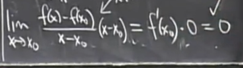 f(x0) = (f(x)-f(x0))/(x-x0)


 872
872

 被折叠的 条评论
为什么被折叠?
被折叠的 条评论
为什么被折叠?
 到【灌水乐园】发言


