np.Linear algebra学习

最新推荐文章于 2023-07-09 14:35:09 发布

weixin_34082789

最新推荐文章于 2023-07-09 14:35:09 发布

阅读量239

点赞数

CC 4.0 BY-SA版权

文章标签： python 人工智能

原文链接：http://www.cnblogs.com/BlueBlueSea/p/10562989.html

本文转自相关文档，介绍了Python numpy库中线性代数的相关内容。包括分解（如svd奇异值分解）、矩阵特征值计算、范数和其他数字（如矩阵范数、条件数、行列式等）的计算，以及解方程和逆矩阵（如线性矩阵方程求解、最小二乘求解）等函数的使用。

转自：https://docs.scipy.org/doc/numpy-1.13.0/reference/routines.linalg.html

1.分解

//其中我觉得可以的就是svd奇异值分解吧，虽然并不知道数学原理

np.linalg.svd(a, full_matrices=1, compute_uv=1)

a是要分解的(M,N)array;

full_matrices : bool, optional

If True (default), u and v have the shapes (M, M) and (N, N), respectively. Otherwise, the shapes are (M, K) and (K, N), respectively, where K = min(M, N).

当full_matrices是True时（默认）：

>>> d=np.mat("4 11 14;8 7 -2")
>>> d
matrix([[ 4, 11, 14],
        [ 8,  7, -2]])
>>> U,sigma,V=np.linalg.svd(d)
>>> U
matrix([[-0.9486833 , -0.31622777],
        [-0.31622777,  0.9486833 ]])
>>> V
matrix([[-0.33333333, -0.66666667, -0.66666667],
        [ 0.66666667,  0.33333333, -0.66666667],
        [-0.66666667,  0.66666667, -0.33333333]])
>>> sigma
array([18.97366596,  9.48683298])
>>> U.shape,sigma.shape,V.shape
((2, 2), (2,), (3, 3))
>>> S=np.zeros((2,3))
>>> S[:2,:2]=np.diag(sigma)
>>> S
array([[18.97366596,  0.        ,  0.        ],
       [ 0.        ,  9.48683298,  0.        ]])
>>> U*S*V
matrix([[ 4., 11., 14.],
        [ 8.,  7., -2.]])

当full_matrices是False时:

>>> U,sigma,V=np.linalg.svd(d,full_matrices=0)
>>> U
matrix([[-0.9486833 , -0.31622777],
        [-0.31622777,  0.9486833 ]])
>>> sigma
array([18.97366596,  9.48683298])
>>> V
matrix([[-0.33333333, -0.66666667, -0.66666667],
        [ 0.66666667,  0.33333333, -0.66666667]])
>>> S=np.diag(sigma)#####
>>> S
array([[18.97366596,  0.        ],
       [ 0.        ,  9.48683298]])
>>> U*S*V
matrix([[ 4., 11., 14.],
        [ 8.,  7., -2.]])

2.矩阵特征值

np.linalg.eig(a) Compute the eigenvalues and right eigenvectors of a square array.

>>> w,v=LA.eig(np.diag((1,2,3)))
>>> w
array([1., 2., 3.])
>>> v
array([[1., 0., 0.],
       [0., 1., 0.],
       [0., 0., 1.]])
>>> np.diag((1,2,3))
array([[1, 0, 0],
       [0, 2, 0],
       [0, 0, 3]])

np.linalg.eigvals(g):Compute the eigenvalues of a general matrix.

>>> w2=LA.eigvals(np.diag((1,2,3)))
>>> w2
array([1., 2., 3.])

3.范数和其他数字

3.1 np.linalg.norm(x, ord=None, axis=None, keepdims=False):Matrix or vector norm.

Using the axis argument to compute vector norms:axis用来计算矩阵中的向量范数。

>>> a=np.array([3,4])
>>> a
array([3, 4])
>>> LA.norm(a)
5.0
>>> LA.norm(a,ord=1)
7.0
>>> a=np.array([3,-4])
>>> LA.norm(a,ord=1)
7.0
>>> LA.norm(a,ord=np.inf)
4.0
>>> LA.norm(a,ord=-np.inf)
3.0

3.2 np.linalg.cond(x, p=None):Compute the condition number of a matrix.

>>> a=np.array([[1, 0, -1], [0, 1, 0], [1, 0, 1]])
>>> a
array([[ 1,  0, -1],
       [ 0,  1,  0],
       [ 1,  0,  1]])
>>> LA.cond(a)
1.4142135623730951
>>> LA.cond(a,2)
1.4142135623730951
>>> LA.cond(a,1)
2.0

//其中：

p : {None, 1, -1, 2, -2, inf, -inf, ‘fro’}, optional

Order of the norm:

p norm for matrices
None 2-norm, computed directly using the SVD
‘fro’ Frobenius norm
inf max(sum(abs(x), axis=1))
-inf min(sum(abs(x), axis=1))
1 max(sum(abs(x), axis=0))
-1 min(sum(abs(x), axis=0))
2 2-norm (largest sing. value)
-2 smallest singular value

inf means the numpy.inf object, and the Frobenius norm is the root-of-sum-of-squares norm.

p	norm for matrices
None	2-norm, computed directly using the `SVD`
‘fro’	Frobenius norm
inf	max(sum(abs(x), axis=1))
-inf	min(sum(abs(x), axis=1))
1	max(sum(abs(x), axis=0))
-1	min(sum(abs(x), axis=0))
2	2-norm (largest sing. value)
-2	smallest singular value

使用的范数，默认是L2范数。

3.3 np.linalg.det(a):Compute the determinant of an array.

>>> a = np.array([[1, 2], [3, 4]])
>>> LA.det(a)
-2.0000000000000004

3.4 np.linalg.matrix_rank(M, tol=None):Return matrix rank of array using SVD method

>>> LA.matrix_rank(np.eye(4))
4
>>> I=np.eye(4)
>>> I[-1,-1]=0
>>> I
array([[1., 0., 0., 0.],
       [0., 1., 0., 0.],
       [0., 0., 1., 0.],
       [0., 0., 0., 0.]])
>>> LA.matrix_rank(I)
3

3.5 trace(a, offset=0, axis1=0, axis2=1, dtype=None, out=None)

>>> np.trace(np.eye(4))
4.0

矩阵对角线上的和。

4.解方程和逆矩阵

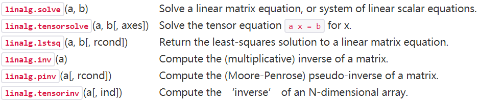
4.1 np.linalg.solve(a,b)：Solve a linear matrix equation, or system of linear scalar equations.

Solve the system of equations 3 * x0 + x1 = 9 and x0 + 2 * x1 = 8:

>>> a = np.array([[3,1], [1,2]])
>>> b = np.array([9,8])
>>> x = np.linalg.solve(a, b)
>>> x
array([ 2.,  3.])

check:

>>> np.allclose(np.dot(a, x), b)
True

4.2 np.linalg.lstsq(a, b, rcond=-1):Return the least-squares solution to a linear matrix equation

最小二乘求解。

转载于:https://www.cnblogs.com/BlueBlueSea/p/10562989.html