线性回归、逻辑回归算法解析，特征选择，交叉验证，sparkmllib

最新推荐文章于 2021-10-16 20:24:55 发布

转载最新推荐文章于 2021-10-16 20:24:55 发布 · 387 阅读

3 ·

CC 4.0 BY-SA版权

原文链接：http://www.cnblogs.com/xiaoma0529/p/6928192.html

文章标签：

#数据结构与算法 #大数据 #java

本文深入探讨了线性回归及逻辑回归的基本原理和技术要点，包括最大似然估计、最小二乘法及其背后的数学原理，并介绍了如何利用Spark进行特征选择与交叉验证。

摘要生成于 C知道，由 DeepSeek-R1 满血版支持，前往体验 >

线性回归、逻辑回归可以解决分类问题(二分类、多分类)、回归问题。

主要技术点

线性回归
 高斯分布
 最大似然估计MLE
 最小二乘法的本质
Logistic回归
 分类问题的首选算法
重要技术
 梯度下降算法
 最大似然估计
 特征选择

 交叉验证

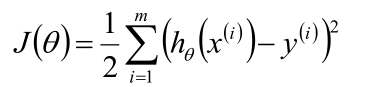
一、线性回归

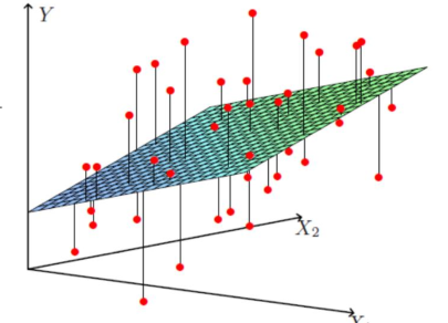
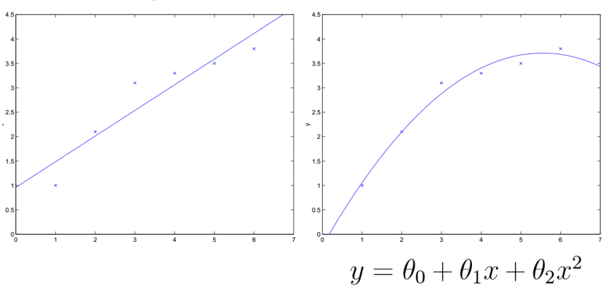
y=ax+b (一个变量)

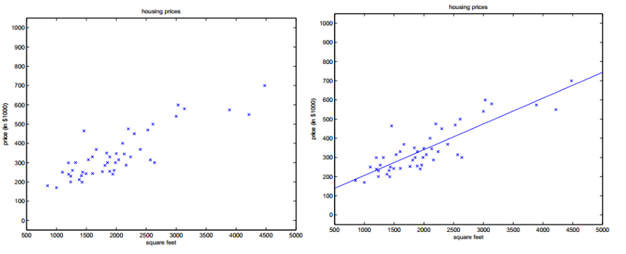
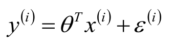
两个变量的情况

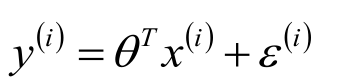
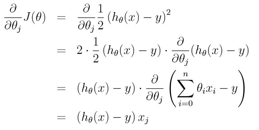
使用极大似然估计解释最小二乘

误差满足中心极限定理

误差ε (i) (1≤i≤m)是独立同分布的，服从均值
为0，方差为某定值σ 2 的高斯分布。

中心极限定理解释

实际问题中，很多随机现象可以看做众多因
素的独立影响的综合反应，往往近似服从正
态分布。
 城市耗电量：大量用户的耗电量总和
 测量误差：许多观察不到的、微小误差的总和

似然函数

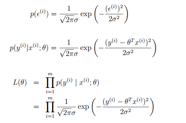
高斯的对数似然

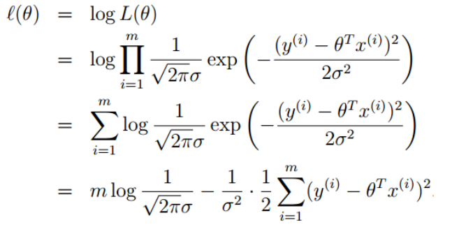
似然函数求最大值相应的

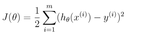
取最小(最小二乘法)

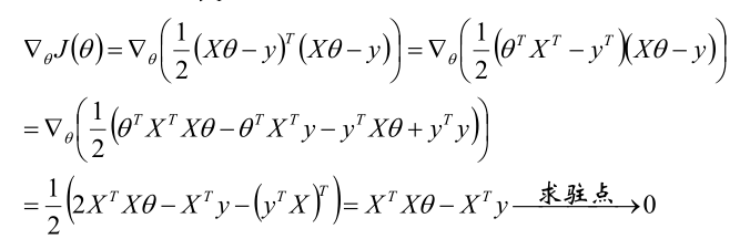
目标函数求解

梯度

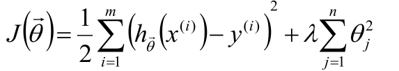
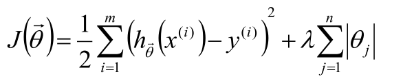
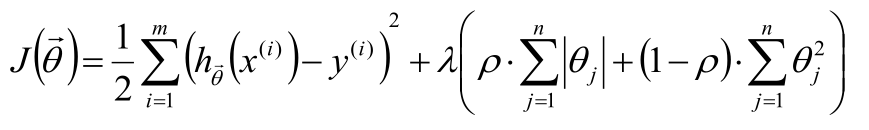
线性回归的复杂度惩罚因子(正则项)

L2正则化

L1正则化

Elastic Net正则化

选取

交叉验证法(三折交叉验证、十折交叉验证)

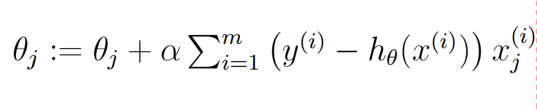
把样本分出一部分验证数据,如三折交叉验证可以分为训练数据-训练数据-验证数据-测试数据

交叉验证

spark中有交叉验证的实现部分

  CrossValidator cv=new CrossValidator()
                .setEstimator(pipeline)
                .setEvaluator(new RegressionEvaluator()
                 .setLabelCol("rating")
                 .setPredictionCol("predict_rating")
                 .setMetricName("rmse"))
                .setEstimatorParamMaps(paramGrid)
                .setNumFolds(5);

梯度下降算法

初始化θ(随机初始化)
 沿着负梯度方向迭代，更新后的θ使J(θ)更小

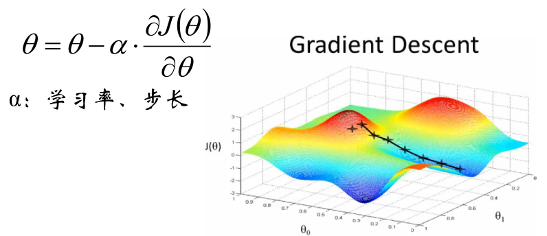
对目标函数求偏导数

批量梯度下降算法

梯度下降有可能找到全局最小值，批量梯度下降会找到局部最小值

特征选择

如特征为x1、x2 输出为y

可以应用提升特征的方法达到更好的效果

特征选择很重要，除了人工选择，还可以用
其他机器学习方法，如随机森林、PCA、
LDA等。

spark代码

LogisticRegression实现   分类同理

import java.io.PrintWriter
import java.util

import org.apache.spark.ml.attribute.{Attribute, AttributeGroup, NumericAttribute}
import org.apache.spark.ml.classification.{BinaryLogisticRegressionTrainingSummary, LogisticRegressionModel, LogisticRegression}
import org.apache.spark.mllib.classification.LogisticRegressionWithSGD
import org.apache.spark.mllib.linalg.Vectors
import org.apache.spark.rdd.RDD
import org.apache.spark.sql.{SQLContext, DataFrame, Row}
import org.apache.spark.sql.types.{DataTypes, StructField}
import org.apache.spark.{SparkContext, SparkConf}

object LogisticRegression {
    def main(args: Array[String]) {
        val conf = new SparkConf().setAppName("test").setMaster("local")
        val sc = new SparkContext(conf)
        val sql  = new SQLContext(sc);
        val training: DataFrame = sql.read.format("libsvm").load("a.txt")

//        val training = sc.read.format("libsvm").load("data/mllib/sample_libsvm_data.txt")

        val data: RDD[String] = sc.textFile("string.txt")
        val rw= data.map{ row =>
            var split: Array[String] = row.split(",")
            Row(split(0).toDouble,Vectors.dense(split(1).toDouble,split(2).toDouble))
        }

        val defaultAttr = NumericAttribute.defaultAttr
        val attrs = Array("f1", "f2").map(defaultAttr.withName)
        val attrGroup = new AttributeGroup("features", attrs.asInstanceOf[Array[Attribute]])
        val  fields = new util.ArrayList[StructField];
        fields.add(DataTypes.createStructField("label", DataTypes.DoubleType, true));
        fields.add(attrGroup.toStructField());


        val structType = DataTypes.createStructType(fields);

        val df: DataFrame = sql.createDataFrame(rw,structType)
        df.printSchema()
        df.show()
        val lr = new LogisticRegression()
                .setMaxIter(10)
                .setRegParam(0.3)
                .setElasticNetParam(1)//默认0 L2   1---》L1

        // Fit the model
        val lrModel: LogisticRegressionModel = lr.fit(df)

        // Print the coefficients and intercept for logistic regression
//        coefficients 系数  intercept 截距
        println(s"Coefficients: ${lrModel.coefficients} Intercept: ${lrModel.intercept}")

        lrModel.write.overwrite().save("F:\\mode")

        val weights: Array[Double] = lrModel.weights.toArray

        val pw = new PrintWriter("F:\\weights");
        //遍历
        for(i<- 0 until weights.length){
            //通过map得到每个下标相应的特征名

            //特征名对应相应的权重
            val str = weights(i)
            pw.write(str.toString)
            pw.println()
        }
        pw.flush()
        pw.close()


    }
}

　　样本数据

0 1:5.1 2:3.5 3:1.4 4:0.2
0 1:4.9 2:3.0 3:1.4 4:0.2
0 1:4.7 2:3.2 3:1.3 4:0.2
0 1:4.6 2:3.1 3:1.5 4:0.2
0 1:5.0 2:3.6 3:1.4 4:0.2
0 1:5.4 2:3.9 3:1.7 4:0.4
0 1:4.6 2:3.4 3:1.4 4:0.3
0 1:5.0 2:3.4 3:1.5 4:0.2
0 1:4.4 2:2.9 3:1.4 4:0.2
0 1:4.9 2:3.1 3:1.5 4:0.1
0 1:5.4 2:3.7 3:1.5 4:0.2
0 1:4.8 2:3.4 3:1.6 4:0.2
0 1:4.8 2:3.0 3:1.4 4:0.1
0 1:4.3 2:3.0 3:1.1 4:0.1
0 1:5.8 2:4.0 3:1.2 4:0.2
0 1:5.7 2:4.4 3:1.5 4:0.4
0 1:5.4 2:3.9 3:1.3 4:0.4
0 1:5.1 2:3.5 3:1.4 4:0.3
0 1:5.7 2:3.8 3:1.7 4:0.3
0 1:5.1 2:3.8 3:1.5 4:0.3
0 1:5.4 2:3.4 3:1.7 4:0.2
0 1:5.1 2:3.7 3:1.5 4:0.4
0 1:4.6 2:3.6 3:1.0 4:0.2
0 1:5.1 2:3.3 3:1.7 4:0.5
0 1:4.8 2:3.4 3:1.9 4:0.2
0 1:5.0 2:3.0 3:1.6 4:0.2
0 1:5.0 2:3.4 3:1.6 4:0.4
0 1:5.2 2:3.5 3:1.5 4:0.2
0 1:5.2 2:3.4 3:1.4 4:0.2
0 1:4.7 2:3.2 3:1.6 4:0.2
0 1:4.8 2:3.1 3:1.6 4:0.2
0 1:5.4 2:3.4 3:1.5 4:0.4
0 1:5.2 2:4.1 3:1.5 4:0.1
0 1:5.5 2:4.2 3:1.4 4:0.2
0 1:4.9 2:3.1 3:1.5 4:0.1
0 1:5.0 2:3.2 3:1.2 4:0.2
0 1:5.5 2:3.5 3:1.3 4:0.2
0 1:4.9 2:3.1 3:1.5 4:0.1
0 1:4.4 2:3.0 3:1.3 4:0.2
0 1:5.1 2:3.4 3:1.5 4:0.2
0 1:5.0 2:3.5 3:1.3 4:0.3
0 1:4.5 2:2.3 3:1.3 4:0.3
0 1:4.4 2:3.2 3:1.3 4:0.2
0 1:5.0 2:3.5 3:1.6 4:0.6
0 1:5.1 2:3.8 3:1.9 4:0.4
0 1:4.8 2:3.0 3:1.4 4:0.3
0 1:5.1 2:3.8 3:1.6 4:0.2
0 1:4.6 2:3.2 3:1.4 4:0.2
0 1:5.3 2:3.7 3:1.5 4:0.2
0 1:5.0 2:3.3 3:1.4 4:0.2
1 1:7.0 2:3.2 3:4.7 4:1.4
1 1:6.4 2:3.2 3:4.5 4:1.5
1 1:6.9 2:3.1 3:4.9 4:1.5
1 1:5.5 2:2.3 3:4.0 4:1.3
1 1:6.5 2:2.8 3:4.6 4:1.5
1 1:5.7 2:2.8 3:4.5 4:1.3
1 1:6.3 2:3.3 3:4.7 4:1.6
1 1:4.9 2:2.4 3:3.3 4:1.0
1 1:6.6 2:2.9 3:4.6 4:1.3
1 1:5.2 2:2.7 3:3.9 4:1.4
1 1:5.0 2:2.0 3:3.5 4:1.0
1 1:5.9 2:3.0 3:4.2 4:1.5
1 1:6.0 2:2.2 3:4.0 4:1.0
1 1:6.1 2:2.9 3:4.7 4:1.4
1 1:5.6 2:2.9 3:3.6 4:1.3
1 1:6.7 2:3.1 3:4.4 4:1.4
1 1:5.6 2:3.0 3:4.5 4:1.5
1 1:5.8 2:2.7 3:4.1 4:1.0
1 1:6.2 2:2.2 3:4.5 4:1.5
1 1:5.6 2:2.5 3:3.9 4:1.1
1 1:5.9 2:3.2 3:4.8 4:1.8
1 1:6.1 2:2.8 3:4.0 4:1.3
1 1:6.3 2:2.5 3:4.9 4:1.5
1 1:6.1 2:2.8 3:4.7 4:1.2
1 1:6.4 2:2.9 3:4.3 4:1.3
1 1:6.6 2:3.0 3:4.4 4:1.4
1 1:6.8 2:2.8 3:4.8 4:1.4
1 1:6.7 2:3.0 3:5.0 4:1.7
1 1:6.0 2:2.9 3:4.5 4:1.5
1 1:5.7 2:2.6 3:3.5 4:1.0
1 1:5.5 2:2.4 3:3.8 4:1.1
1 1:5.5 2:2.4 3:3.7 4:1.0
1 1:5.8 2:2.7 3:3.9 4:1.2
1 1:6.0 2:2.7 3:5.1 4:1.6
1 1:5.4 2:3.0 3:4.5 4:1.5
1 1:6.0 2:3.4 3:4.5 4:1.6
1 1:6.7 2:3.1 3:4.7 4:1.5
1 1:6.3 2:2.3 3:4.4 4:1.3
1 1:5.6 2:3.0 3:4.1 4:1.3
1 1:5.5 2:2.5 3:4.0 4:1.3
1 1:5.5 2:2.6 3:4.4 4:1.2
1 1:6.1 2:3.0 3:4.6 4:1.4
1 1:5.8 2:2.6 3:4.0 4:1.2
1 1:5.0 2:2.3 3:3.3 4:1.0
1 1:5.6 2:2.7 3:4.2 4:1.3
1 1:5.7 2:3.0 3:4.2 4:1.2
1 1:5.7 2:2.9 3:4.2 4:1.3
1 1:6.2 2:2.9 3:4.3 4:1.3
1 1:5.1 2:2.5 3:3.0 4:1.1
1 1:5.7 2:2.8 3:4.1 4:1.3
2 1:6.3 2:3.3 3:6.0 4:2.5
2 1:5.8 2:2.7 3:5.1 4:1.9
2 1:7.1 2:3.0 3:5.9 4:2.1
2 1:6.3 2:2.9 3:5.6 4:1.8
2 1:6.5 2:3.0 3:5.8 4:2.2
2 1:7.6 2:3.0 3:6.6 4:2.1
2 1:4.9 2:2.5 3:4.5 4:1.7
2 1:7.3 2:2.9 3:6.3 4:1.8
2 1:6.7 2:2.5 3:5.8 4:1.8
2 1:7.2 2:3.6 3:6.1 4:2.5
2 1:6.5 2:3.2 3:5.1 4:2.0
2 1:6.4 2:2.7 3:5.3 4:1.9
2 1:6.8 2:3.0 3:5.5 4:2.1
2 1:5.7 2:2.5 3:5.0 4:2.0
2 1:5.8 2:2.8 3:5.1 4:2.4
2 1:6.4 2:3.2 3:5.3 4:2.3
2 1:6.5 2:3.0 3:5.5 4:1.8
2 1:7.7 2:3.8 3:6.7 4:2.2
2 1:7.7 2:2.6 3:6.9 4:2.3
2 1:6.0 2:2.2 3:5.0 4:1.5
2 1:6.9 2:3.2 3:5.7 4:2.3
2 1:5.6 2:2.8 3:4.9 4:2.0
2 1:7.7 2:2.8 3:6.7 4:2.0
2 1:6.3 2:2.7 3:4.9 4:1.8
2 1:6.7 2:3.3 3:5.7 4:2.1
2 1:7.2 2:3.2 3:6.0 4:1.8
2 1:6.2 2:2.8 3:4.8 4:1.8
2 1:6.1 2:3.0 3:4.9 4:1.8
2 1:6.4 2:2.8 3:5.6 4:2.1
2 1:7.2 2:3.0 3:5.8 4:1.6
2 1:7.4 2:2.8 3:6.1 4:1.9
2 1:7.9 2:3.8 3:6.4 4:2.0
2 1:6.4 2:2.8 3:5.6 4:2.2
2 1:6.3 2:2.8 3:5.1 4:1.5
2 1:6.1 2:2.6 3:5.6 4:1.4
2 1:7.7 2:3.0 3:6.1 4:2.3
2 1:6.3 2:3.4 3:5.6 4:2.4
2 1:6.4 2:3.1 3:5.5 4:1.8
2 1:6.0 2:3.0 3:4.8 4:1.8
2 1:6.9 2:3.1 3:5.4 4:2.1
2 1:6.7 2:3.1 3:5.6 4:2.4
2 1:6.9 2:3.1 3:5.1 4:2.3
2 1:5.8 2:2.7 3:5.1 4:1.9
2 1:6.8 2:3.2 3:5.9 4:2.3
2 1:6.7 2:3.3 3:5.7 4:2.5
2 1:6.7 2:3.0 3:5.2 4:2.3
2 1:6.3 2:2.5 3:5.0 4:1.9
2 1:6.5 2:3.0 3:5.2 4:2.0
2 1:6.2 2:3.4 3:5.4 4:2.3
2 1:5.9 2:3.0 3:5.1 4:1.8

转载于:https://www.cnblogs.com/xiaoma0529/p/6928192.html