Constructing GLMs

1. Guide

　　More generally, consider a classification or regression problem where we would like to predict the value of some random variable y as a function of x. To derive a GLM for this problem, we will make the following three assumptions about the conditional distribution of y given x and about our model:

　　a. y | x; θ ∼ ExponentialFamily(η). I.e., given x and θ, the distribution of y follows some exponential family distribution, with parameter η.

　　b. Given x, our goal is to predict the expected value of T(y) given x. In most of our examples, we will have T(y) = y, so this means we would like the prediction h(x) output by our learned hypothesis h to satisfy h_θ(x) = E[y|x]. (Note that this assumption is satisfied in the choices for h(x) for both logistic regression and linear regression. For instance, in logistic regression, we had h_θ(x) = p(y = 1|x; θ) = 0 · p(y = 0|x; θ) + 1 · p(y = 1|x; θ) = E[y|x; θ].)

　　c. The natural parameter η and the inputs x are related linearly: η = θ^Tx. (if η is vector-valued, then η_i = θ_i^Tx. θ=(θ₁, θ₂,...θ_k)^T, θ₁, θ₂,...θ_k are all n+1-vectors, the target variable y will be k-vector)

　　---These three assumptions/design choices will allow us to derive a very elegant class of learning algorithms, namely GLMs, that have many desirable properties such as ease of learning.

 

2. Ordinary Least Squares

　　Consider the setting where the target variable y (also called the response variable in GLM terminology) is continuous, and we model the conditional distribution of y given x as as a Gaussian N(μ, σ²).

　　　　h(x) = E[y|x; θ]= μ = η = θ^T x.

 

3. Logistic Regression

　　Here we are interested in binary classification, so y ∈ {0, 1}. Given that y is binary-valued, it therefore seems natural to choose the Bernoulli family of distributions to model the conditional distribution of y given x.

　　　　h(x) = E[y|x; θ]= φ = 1/(1 + e^−η) = 1/(1 + e^{−θT x})

　　You are previously wondering how we came up with the form of the logistic function 1/(1 + e^−z), this gives one answer: Once we assume that y conditioned on x is Bernoulli, it arises as a consequence of the definition of GLMs and exponential family distributions.

　　Note: To introduce a little more terminology, the function g giving the distribution’s mean as a function of the natural parameter (g(η) = E[T(y); η]) is called the canonical response function. Its inverse, g⁻¹, is called the canonical link function. Thus, the canonical response function for the Gaussian family is just the identify function; and the canonical response function for the Bernoulli is the logistic function.

 

4. Softmax Regression

　　Consider a classification problem in which the response variable y can take on any one of k values, so y ∈ {1 2, . . . , k}.

　　To parameterize a multinomial over k possible outcomes, one could use k - 1parameters φ₁, . . . , φ_k-1 specifying the probability of each of the outcomes.

　　For notational convenience, we will let φ_k = 1 − φ₁ − φ₂ − ... − φ_k-1, but we should keep in mind that this is not a parameter, and that it is fully specified by φ₁, . . . , φ_k−1.

　　To express the multinomial as an exponential family distribution, we will define T(y) ∈ R^k−1 as follows:

　　　　

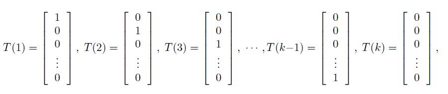
　　T(y) is now a k − 1 dimensional vector, rather than a real number. We will write (T(y))_i to denote the i-th element of the vector T(y).

　　We introduce one more very useful piece of notation. An indicator function 1{·} takes on a value of 1 if its argument is true, and 0 otherwise. For example, 1{2 = 3} = 0, and 1{3 = 5 − 2} = 1.So, we can also write the relationship between T(y) and y as (T(y))_i = 1{y = i}.

　　We have that E[(T(y))_i] = P(y = i) = φ_i.

　　We are now ready to show that the multinomial is a member of the exponential family. We have:

　　　　

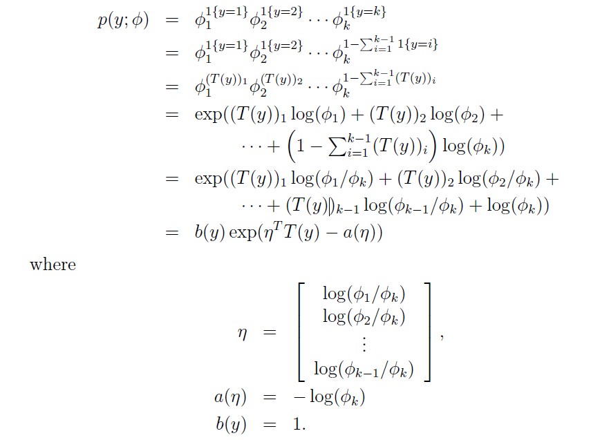
　　This completes our formulation of the multinomial as an exponential family distribution.

　　The link function is given (for i = 1, . . . , k) by

　　　　η_i = log(φ_i/φ_k)

　　For convenience, we have also defined η_k = log(φ_k/φ_k) = 0.

　　To invert the link function and derive the response function, we therefore have that:

　　　　

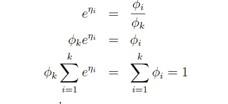
　　This will be:

　　　　

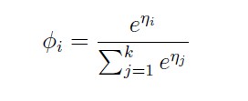
　　To complete our model, we use Assumption 3, given earlier, that the η_i’s are linearly related to the x’s. So, have η_i = θ_i^Tx (for i = 1, . . . , k − 1), where θ₁, . . . , θ_k−1 ∈ Rⁿ⁺¹ are the parameters of our model. For notational convenience, we can also define θ_k = 0, so that η_k = θ_k^Tx = 0, as given previously. Hence, our model assumes that the conditional distribution of y given x is given by

　　　　

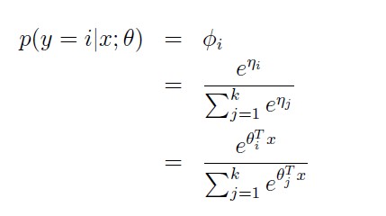
　　This model, which applies to classification problems where y ∈ {1, . . . , k}, is called softmax regression. It is a generalization of logistic regression.

　　Our hypothesis will output:

　　　　

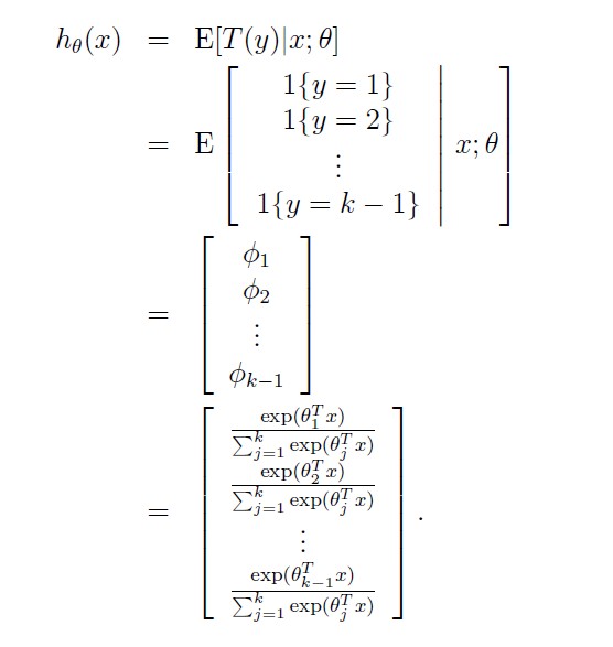
　　In other words, our hypothesis will output the estimated probability that p(y = i|x; θ), for every value of i = 1, . . . , k. (Even though h_θ(x) as defined above is only k − 1 dimensional, clearly p(y = k|x; θ) can be obtained as 1 − φ₁ − φ₂ − ... − φ_k-1)

　　Lastly, lets discuss parameter fitting. Similar to our original derivation of ordinary least squares and logistic regression, if we have a training set of m examples {(x⁽ⁱ⁾, y⁽ⁱ⁾); i = 1, . . . ,m} and would like to learn the parameters θ_i of this model, we would begin by writing down the log-likelihood:

　　　　

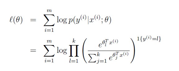
　　We can now obtain the maximum likelihood estimate of the parameters by maximizing l(θ) in terms of θ, using a method such as gradient ascent or Newton’s method.Here, θ is θ₁,θ₂,...,θ_k-1 are all n+1-vector.

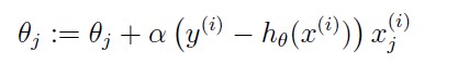
　　Note: We can obtain for all GLM Models update rule like:

　　　　　　

　　　　

转载于:https://www.cnblogs.com/ustccjw/archive/2013/04/14/3020177.html