LMS算法详解-优快云博客

最小均方算法（LMS Algorithm）及其matlab代码实现

　　线性回归的目的是寻找θ使得J(θ)取得最小值。如何使J(θ)取得最小值，可以采用梯度下降算法逐步逼近。

　　算法过程如下：

　　（1）初始化一个θ，可以取随机值；

　　（2）采用如下公式进行迭代：

　　　　　　 $\theta_{j} := \theta_{j} - \alpha \frac{\partial }{\partial \theta_{j}} J(\theta)$

　　　　其中，θ_j是θ的第j个分量，α是步长，也称为学习速率（Learning rate）。最后那一部分是J(θ)关于θ_j的导数。

　　对于只有一个训练样本的情况，我们有：

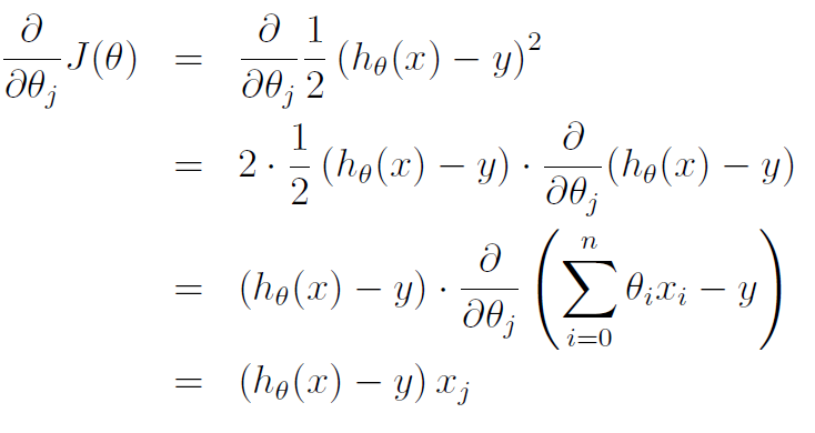
　　由此，可以得到一个训练样本时的更新规则：

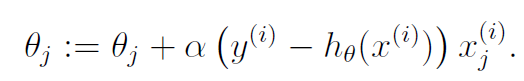
　　　　这个规则称为LMS更新规则，也叫做Widrow-Hoff学习规则。上标i表示第i个训练样本，不是指数。

　　对于一个训练集来说，有两种更新的策略：

　　　　第一种，称之为批量梯度下降法，就是说每一次更新时，都要涉及所有的样本。更新公式如下：

　　　　公式中，m为训练样本的数目。参考一个训练样本的更新规则，可以很明显的看到，批量梯度下降算法是在每一轮迭代中，所有的训练样本更新规则相叠加。

　　　　第二种，称之为随机梯度下降法，就是说在每训练一个样本时，都进行一次更新操作。更新操作如下：

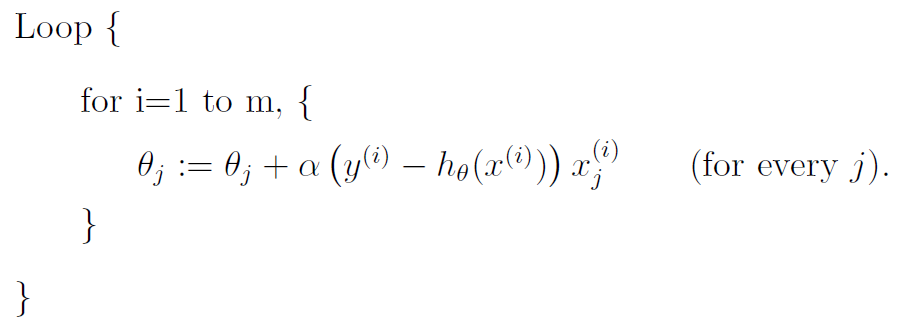
　　　　随机梯度下降法相对于批量梯度下降算法来说，它不用每次更新都把所有的训练样本都计算一遍，它的更新速度比批量梯度下降算法更快，消耗的内存更少。当然，随机梯度下降法每一次更新完成后，结果不一定会变得更好，甚至会变得更坏，但总体趋势是梯度下降的。当样本的数目m很大时，随机梯度下降法能更好的解决问题。

以下是批量梯度下降算法的matlab实现：

%LinRegTrain function is used to train data for linear regression.
%FEATURE is the matrix that composed of features of the training examples.
%VALUE is the matrix that composed of output values of the training
%examples.
%THETA is the parameter of the hypotheses function.
function [theta] = LinRegTrain(feature,value)
length = size(feature,2);
num = size(feature,1);
features = [ones(num,1) feature];
theta = zeros(length + 1,1);
alpha = 0.005/(num*10);
%theta = 1 + rand(1,length + 1);
for i = 1:100000;
　　delta = value - features*theta;
% 　　 costvalue = delta'*delta;
% 　　 if costvalue < 1e-10;
% 　　 display 'break the if condition'
% 　　 break;
% 　　 end
　　theta = theta + alpha*features'*delta;
% 　　 theta(1) = theta(1) + alpha*sum(delta.*features(:,1));
% 　　 theta(2) = theta(2) + alpha*sum(delta.*features(:,2));
end
hypvalue = features*theta;
plot(feature,hypvalue,'rx-',feature,value,'bo');
end