


 本文介绍了NumPy和Pandas的基础用法,包括数组创建、基本运算、索引选取及DataFrame的操作等内容。通过实例展示了如何使用这些库进行数据处理。
numpy基础
import numpy as np定义array
In [156]: np.ones(3)
Out[156]: array([1., 1., 1.])

In [157]: np.ones((3,5))
Out[157]:
array([[1., 1., 1., 1., 1.],
       [1., 1., 1., 1., 1.],
       [1., 1., 1., 1., 1.]])

In [158]:

In [158]: np.zeros(4)
Out[158]: array([0., 0., 0., 0.])

In [159]: np.zeros((2,5))
Out[159]:
array([[0., 0., 0., 0., 0.],
       [0., 0., 0., 0., 0.]])

In [160]:
In [146]: a = np.array([[1,3,5,2],[4,2,6,1]])

In [147]: print(a)
[[1 3 5 2]
 [4 2 6 1]]

In [148]:
In [161]: np.arange(10)
Out[161]: array([0, 1, 2, 3, 4, 5, 6, 7, 8, 9])

In [162]: np.arange(3,13)
Out[162]: array([ 3,  4,  5,  6,  7,  8,  9, 10, 11, 12])

In [163]: np.arange(3,13).reshape((2,5))
Out[163]:
array([[ 3,  4,  5,  6,  7],
       [ 8,  9, 10, 11, 12]])

In [164]:
In [169]: np.arange(2,25,2)
Out[169]: array([ 2,  4,  6,  8, 10, 12, 14, 16, 18, 20, 22, 24])

In [170]: np.arange(2,25,2).reshape(3,4)
Out[170]:
array([[ 2,  4,  6,  8],
       [10, 12, 14, 16],
       [18, 20, 22, 24]])

In [171]:

In [176]:  np.linspace(1,10,4)
Out[176]: array([ 1.,  4.,  7., 10.])

In [177]:
array基本运算
In [7]: a = np.array([[1,2],[3,4]])

In [8]: b = np.arange(5,9).reshape((2,3))
In [10]: print(a)
[[1 2]
 [3 4]]

In [11]: print(b)
[[5 6]
 [7 8]]

In [12]:

In [12]: a+b
Out[12]:
array([[ 6,  8],
       [10, 12]])

In [13]: a-b
Out[13]:
array([[-4, -4],
       [-4, -4]])

In [14]: a*b     # 对应元素相乘
Out[14]:
array([[ 5, 12],
       [21, 32]])

In [17]: a/b
Out[17]:
array([[0, 0],
       [0, 0]])

In [18]:

In [18]: a**2
Out[18]:
array([[ 1, 4],
[ 9, 16]])

In [19]:


In [15]: np.dot(a,b)   # 矩阵乘法
Out[15]:
array([[19, 22],
[43, 50]])

In [16]: a.dot(b)
Out[16]:
array([[19, 22],
[43, 50]])

In [17]:


In [54]: print(a)
[[ 2  3  4  5]
 [ 6  7  8  9]
 [10 11 12 13]]

In [55]: np.sum(a)
Out[55]: 90

In [56]: np.min(a)
Out[56]: 2

In [57]: np.max(a)
Out[57]: 13

In [58]:

In [58]: np.sum(a,axis=1)
Out[58]: array([14, 30, 46])

In [59]: np.sum(a,axis=0)
Out[59]: array([18, 21, 24, 27])

In [60]:


# 三角函数结合random生成一组随机数据
In [74]: N = 10

In [75]: t = np.linspace(0, 2*np.pi, N)

In [76]: print(t)
[0.         0.6981317  1.3962634  2.0943951  2.7925268  3.4906585
 4.1887902  4.88692191 5.58505361 6.28318531]

In [77]: y = np.sin(t) + 0.02*np.random.randn(N)

In [78]: print(y)
[-0.00947902  0.64196198  0.96567468  0.89394571  0.33830193 -0.3015316
 -0.86943758 -0.95954123 -0.62526393  0.02872202]

In [79]: M = 3

In [80]: for ii, vv in zip(np.random.rand(M)*N, np.random.randn(M)):
    ...:     y[int(ii):] += vv
    ...:

In [81]: print(y)
[-0.00947902  0.64196198  1.47685437  1.55309848  0.99745469  0.35762117
 -0.21028481 -0.30038846 -0.29746375  0.35652221]

In [82]:


In [101]: a = np.arange(2,14).reshape((3,4))

In [102]: print(a)
[[ 2  3  4  5]
 [ 6  7  8  9]
 [10 11 12 13]]

In [103]: print(np.argmin(a))  # 最小值的索引
0

In [104]: print(np.argmax(a))  # 最大值的索引
11

In [105]: np.cumsum(a)         # 从0元素开始的累计和
Out[105]: array([ 2,  5,  9, 14, 20, 27, 35, 44, 54, 65, 77, 90])

In [106]: np.cumprod(a)        # 从1元素开始的累计乘
Out[106]:
array([         2,          6,         24,        120,        720,
             5040,      40320,     362880,    3628800,   39916800,
        479001600, 6227020800])

In [107]:
In [129]: a
Out[129]:
array([[ 2,  3,  4,  5],
       [ 6,  7,  8,  9],
       [10, 11, 12, 13]])

In [130]: np.cumsum(a,axis=1)
Out[130]:
array([[ 2,  5,  9, 14],
       [ 6, 13, 21, 30],
       [10, 21, 33, 46]])

In [131]: np.cumsum(a,axis=0)
Out[131]:
array([[ 2,  3,  4,  5],
       [ 8, 10, 12, 14],
       [18, 21, 24, 27]])

In [132]:
In [133]: np.cumprod(a,axis=1)
Out[133]:
array([[    2,     6,    24,   120],
       [    6,    42,   336,  3024],
       [   10,   110,  1320, 17160]])

In [134]: np.cumprod(a,axis=0)
Out[134]:
array([[  2,   3,   4,   5],
       [ 12,  21,  32,  45],
       [120, 231, 384, 585]])

In [135]:


In [146]: a = np.array([[1,3,5,2],[4,2,6,1]])

In [147]: print(a)
[[1 3 5 2]
 [4 2 6 1]]

In [148]: a.shape
Out[148]: (2, 4)

In [149]: a.ndim
Out[149]: 2

In [150]: a.size
Out[150]: 8

In [151]: np.diff(a)      # 累差运算
Out[151]:
array([[ 2,  2, -3],
       [-2,  4, -5]])

In [152]: np.diff(a,axis=1)
Out[152]:
array([[ 2,  2, -3],
       [-2,  4, -5]])

In [153]: np.diff(a,axis=0)
Out[153]: array([[ 3, -1,  1, -1]])

In [154]:


In [108]: a = np.array([10,7,11,9,8,13,12,9])

In [109]: a.ndim
Out[109]: 1

In [110]: a.shape
Out[110]: (8,)

In [111]: a.size
Out[111]: 8

In [112]: a.mean()      # 均值
Out[112]: 9.875

In [113]: a.var()       # 方差
Out[113]: 3.609375

In [114]: a.std()       # 标准差
Out[114]: 1.899835519196333

In [115]:
In [117]: np.median(a)  # 中位数
Out[117]: 9.5

In [118]:
In [138]: z = (a-a.mean())/a.std()   # z-score

In [139]: print(z)
[ 0.06579517 -1.5132889   0.59215653 -0.46056619 -0.98692754  1.64487924
  1.11851788 -0.46056619]

In [140]:


In [198]: a = np.arange(-3,3).reshape((2,3))

In [199]: a
Out[199]:
array([[-3, -2, -1],
       [ 0,  1,  2]])

In [200]: np.nonzero(a)  # 查找非0元素
Out[200]: (array([0, 0, 0, 1, 1]), array([0, 1, 2, 1, 2]))

In [201]: print(np.nonzero(a))
(array([0, 0, 0, 1, 1]), array([0, 1, 2, 1, 2]))

In [202]:


In [207]: a = np.arange(14,2,-1).reshape((3,4))

In [208]: print(a)
[[14 13 12 11]
 [10  9  8  7]
 [ 6  5  4  3]]

In [209]: np.sort(a)     # 排序
Out[209]:
array([[11, 12, 13, 14],
       [ 7,  8,  9, 10],
       [ 3,  4,  5,  6]])

In [210]:

In [210]: np.sort(a,axis=1)
Out[210]:
array([[11, 12, 13, 14],
       [ 7,  8,  9, 10],
       [ 3,  4,  5,  6]])

In [211]: np.sort(a,axis=0)
Out[211]:
array([[ 6,  5,  4,  3],
       [10,  9,  8,  7],
       [14, 13, 12, 11]])

In [212]:


# 矩阵的转置
In [212]: a = np.arange(14,2,-1).reshape((3,4))

In [213]: print(a)
[[14 13 12 11]
 [10  9  8  7]
 [ 6  5  4  3]]

In [214]:

In [215]: print(np.transpose(a))
[[14 10  6]
 [13  9  5]
 [12  8  4]
 [11  7  3]]

In [216]: a.T
Out[216]:
array([[14, 10,  6],
       [13,  9,  5],
       [12,  8,  4],
       [11,  7,  3]])

In [217]:

In [220]: a.T.dot(a)  # 先转置,再进行矩阵乘法
Out[220]:
array([[332, 302, 272, 242],
       [302, 275, 248, 221],
       [272, 248, 224, 200],
       [242, 221, 200, 179]])

In [221]:


# 矩阵的clip,处理最大值和最小值
In [221]: print(a)
[[14 13 12 11]
 [10  9  8  7]
 [ 6  5  4  3]]

In [222]: np.clip(a,5,11)
Out[222]:
array([[11, 11, 11, 11],
       [10,  9,  8,  7],
       [ 6,  5,  5,  5]])

In [223]:
卷积运算
numpy.convolve(weights,array)

weight = [a,b,c]
array = [i,j,k,m,n]

Result:[ai, bi+aj, ci+bj+ak, cj+bk+am, ck+bm+an, cm+bn, cn][N-1:-N+1]


针对移动平均算法来预测下一个数据,越接近待预测点的数据权重越大,
那么就需要让 i, j, k, m, n 的系数逐渐增大即可;即让 a > b > c ,并且 a+b+c=1 。


示例:
In [223]: weight = np.ones(3)/3

In [224]: print(weight)
[0.33333333 0.33333333 0.33333333]

In [225]: arr = np.array([8,11,9,7,10])

In [226]: np.convolve(weight,arr)
Out[226]:
array([2.66666667, 6.33333333, 9.33333333, 9.        , 8.66666667,
       5.66666667, 3.33333333])

In [227]:

In [227]: weight = np.array([0.8,0.1,0.1])

In [228]: np.convolve(weight,arr)
Out[228]: array([6.4, 9.6, 9.1, 7.6, 9.6, 1.7, 1. ])

In [229]:
random常用操作
# 生成随机浮点数,范围是在0.0~1.0之间
In [19]: a = np.random.random((2,3))

In [20]: print(a)
[[0.02185901 0.69585563 0.04555439]
 [0.37331857 0.32903986 0.62448246]]

In [21]:

# 生成随机整数,可指定起止范围
In [48]: np.random.randint(3)
Out[48]: 2

In [49]: np.random.randint(low=3,high=9)
Out[49]: 6

In [50]: np.random.randint(low=3,high=9,size=(3,4))
Out[50]:
array([[5, 6, 7, 8],
       [8, 7, 3, 8],
       [5, 4, 5, 5]])

In [51]:
In [68]: np.random.randint(low=-5,high=2,size=(3,4))
Out[68]:
array([[-4, -4, -2,  1],
       [ 1,  0,  0,  1],
       [-4, -3,  1, -5]])

In [69]:

# 生成正态分布,又名高斯分布(Gaussian distribution)随机数
In [64]: np.random.normal()
Out[64]: -0.5399414561419419

In [65]: np.random.normal(loc=0,scale=1,size=(2,3))
Out[65]:
array([[-0.50318082, -0.38614219,  0.30450427],
       [ 0.41711087,  0.29990928, -0.7843322 ]])

In [66]:
In [66]: np.random.normal(loc=2,scale=3,size=(2,3))
Out[66]:
array([[ 3.37067379,  6.23517315,  2.3267659 ],
       [ 6.46832646, -2.76363304,  5.77883853]])

In [67]:

# 生成标准正态分布("standard normal" distribution)随机数,标准正态分布的平均值为0,方差为1,服从u(0,1)分布。
In [83]: np.random.randn()
Out[83]: 0.502482341264108

In [84]: np.random.randn(3,4)
Out[84]:
array([[ 0.34507555, -0.26868132, -0.56103417,  0.86176617],
       [-0.16535555, -0.38045904,  0.48176385, -1.09005206],
       [-0.60780266,  1.74113117, -0.72427329, -0.51232408]])

In [85]:

# 生成[0, 1)间随机数
In [99]: np.random.rand()
Out[99]: 0.607701127768974

In [100]: np.random.rand(3,4)
Out[100]:
array([[0.73020695, 0.53993878, 0.46693879, 0.82611629],
       [0.76117076, 0.16522599, 0.85129611, 0.74448772],
       [0.6450236 , 0.49994053, 0.04115063, 0.30081311]])

In [101]:
array索引
# 一维数组的索引和list类似
略

# 二维数组的索引
In [13]: import numpy as np

In [14]: a = np.arange(3,15).reshape((3,4))

In [15]: print(a)
[[ 3  4  5  6]
 [ 7  8  9 10]
 [11 12 13 14]]

In [16]: a[1]
Out[16]: array([ 7,  8,  9, 10])

In [17]: a[1,2]
Out[17]: 9

In [18]: a[1][2]              # 等价于 a[1,2]
Out[18]: 9

In [19]:

In [19]: a[1,1:-1]            # 获取第二行,除去首尾元素
Out[19]: array([8, 9])

In [20]: a[1,1:2]             # 获取第二行第二个元素
Out[20]: array([8])

In [21]:
In [24]: a[1:-1,2]            # 获取第二列,除去首尾元素
Out[24]: array([9])

In [26]: a[:,2]               # 获取第二列元素
Out[26]: array([ 5,  9, 13])

In [27]:
迭代array
# 迭代行
In [27]: print(a)
[[ 3  4  5  6]
 [ 7  8  9 10]
 [11 12 13 14]]

In [28]: for row in a:
    ...:     print(row)
    ...:
[3 4 5 6]
[ 7  8  9 10]
[11 12 13 14]

In [29]:

# 迭代列
In [29]: print(a.T)
[[ 3  7 11]
 [ 4  8 12]
 [ 5  9 13]
 [ 6 10 14]]

In [30]: for column in a.T:
    ...:     print(column)
    ...:
[ 3  7 11]
[ 4  8 12]
[ 5  9 13]
[ 6 10 14]

In [31]:


# 二维矩阵,多行转换成一行,迭代每一个item
In [31]: print(a)
[[ 3  4  5  6]
 [ 7  8  9 10]
 [11 12 13 14]]

In [32]: print(a.flat)
<numpy.flatiter object at 0x7f392e3545c0>

In [33]: print(a.flatten())
[ 3  4  5  6  7  8  9 10 11 12 13 14]

In [34]: for item in a.flat:
    ...:     print(item)
    ...:
3
4
5
6
7
8
9
10
11
12
13
14

In [35]:
合并array
In [39]: a = np.array([1,2,3])

In [40]: b = np.array([2,2,2])

In [41]: c = np.vstack((a,b))     # vertical stack,上下合并

In [42]: print(c)
[[1 2 3]
 [2 2 2]]

In [43]: c.shape
Out[43]: (2, 3)

In [44]: c.ndim
Out[44]: 2

In [45]: c.size
Out[45]: 6

In [46]:


In [47]: d = np.hstack((a,b))     # horizontal stack,左右合并

In [48]: print(d)
[1 2 3 2 2 2]

In [49]: d.shape
Out[49]: (6,)

In [50]: d.ndim
Out[50]: 1

In [51]: d.size
Out[51]: 6

In [52]:


# newaxis改变数组维度
In [54]: print(a)
[1 2 3]

In [55]: e = a[np.newaxis,:]

In [56]: print(e)
[[1 2 3]]

In [57]: f = a[:,np.newaxis]

In [58]: print(f)
[[1]
 [2]
 [3]]

In [59]:


In [59]: a = np.array([1,2,3])[:,np.newaxis]

In [60]: b = np.array([2,2,2])[:,np.newaxis]

In [61]: print(a)
[[1]
 [2]
 [3]]

In [62]: print(b)
[[2]
 [2]
 [2]]

In [63]: c = np.vstack((a,b))

In [64]: print(c)
[[1]
 [2]
 [3]
 [2]
 [2]
 [2]]

In [65]: d = np.hstack((a,b))        # 合并两个array

In [66]: print(d)
[[1 2]
 [2 2]
 [3 2]]

In [67]:
In [74]: d = np.hstack((a,b,b,a))    # 合并多个array

In [75]: print(d)
[[1 2 2 1]
 [2 2 2 2]
 [3 2 2 3]]

In [76]:


# concatenate 常用来合并多个矩阵或序列,axis可以方便的指定维度
In [76]: a = np.array([1,2,3])

In [77]: b = np.array([2,2,2])

In [78]: a = a[:,np.newaxis]

In [79]: b = b[:,np.newaxis]

In [80]: c = np.concatenate((a,b,b,a),axis=0)

In [81]: print(c)
[[1]
 [2]
 [3]
 [2]
 [2]
 [2]
 [2]
 [2]
 [2]
 [1]
 [2]
 [3]]

In [82]: c = np.concatenate((a,b,b,a),axis=1)

In [83]: print(c)
[[1 2 2 1]
 [2 2 2 2]
 [3 2 2 3]]

In [84]:
分割array
In [92]: a = np.arange(12).reshape((3,4))

In [93]: print(a)
[[ 0  1  2  3]
 [ 4  5  6  7]
 [ 8  9 10 11]]

In [94]: c = np.split(a,2,axis=1)               # 等项分割

In [95]: len(c)
Out[95]: 2

In [96]: c[0]
Out[96]:
array([[0, 1],
       [4, 5],
       [8, 9]])

In [97]: c[1]
Out[97]:
array([[ 2,  3],
       [ 6,  7],
       [10, 11]])

In [98]:

In [98]: print(c)
[array([[0, 1],
       [4, 5],
       [8, 9]]), array([[ 2,  3],
       [ 6,  7],
       [10, 11]])]

In [99]:


In [99]: d = np.array_split(a,3,axis=1)         # 不等项分割

In [100]: len(d)
Out[100]: 3

In [101]: print(d)
[array([[0, 1],
       [4, 5],
       [8, 9]]), array([[ 2],
       [ 6],
       [10]]), array([[ 3],
       [ 7],
       [11]])]

In [102]: d[0]
Out[102]:
array([[0, 1],
       [4, 5],
       [8, 9]])

In [103]: d[1]
Out[103]:
array([[ 2],
       [ 6],
       [10]])

In [104]: d[2]
Out[104]:
array([[ 3],
       [ 7],
       [11]])

In [105]:


In [111]: print(a)
[[ 0  1  2  3]
 [ 4  5  6  7]
 [ 8  9 10 11]]

In [112]: b = np.hsplit(a,2)          # horizontal split,水平分割

In [113]: print(b)
[array([[0, 1],
       [4, 5],
       [8, 9]]), array([[ 2,  3],
       [ 6,  7],
       [10, 11]])]

In [114]: b[0]
Out[114]:
array([[0, 1],
       [4, 5],
       [8, 9]])

In [115]: b[1]
Out[115]:
array([[ 2,  3],
       [ 6,  7],
       [10, 11]])

In [116]:

In [116]: c = np.vsplit(a,3)          # vertical split,垂直分割

In [117]: len(c)
Out[117]: 3

In [118]: print(c)
[array([[0, 1, 2, 3]]), array([[4, 5, 6, 7]]), array([[ 8,  9, 10, 11]])]

In [119]: c[0]
Out[119]: array([[0, 1, 2, 3]])

In [120]: c[1]
Out[120]: array([[4, 5, 6, 7]])

In [121]: c[2]
Out[121]: array([[ 8,  9, 10, 11]])

In [122]:
Numpy.copy()
In [150]: a = np.arange(4)

In [151]: print(a)
[0 1 2 3]

In [152]: b = a

In [153]: b is a
Out[153]: True

In [154]: a[0] = 99

In [155]: print(b)
[99  1  2  3]

In [156]:

In [156]: c = a.copy()      # deep copy

In [157]: c is a
Out[157]: False

In [159]: print(a)
[99  1  2  3]

In [160]: a[1:3] = [7,8]

In [161]: print(a)
[99  7  8  3]

In [163]: print(b)
[99  7  8  3]

In [164]: print(c)
[99  1  2  3]

In [165]:
Numpy其他
In [169]: a = np.array([-9,7,12,-4,-3,6,2])

In [170]: print(a)
[-9  7 12 -4 -3  6  2]

In [171]: np.abs(a)
Out[171]: array([ 9,  7, 12,  4,  3,  6,  2])

In [172]: np.where(np.abs(a)>6)
Out[172]: (array([0, 1, 2]),)

In [173]:
numpy参考:http://pda.readthedocs.io/en/latest/chp4.html
Pandas基础
import pandas as pdSeries
In [173]: import pandas as pd
In [174]: import numpy as np
In [175]: s = pd.Series([1,3,6,np.nan,44,1]) # 定义pandas.Series
In [176]: print(s)
0 1.0
1 3.0
2 6.0
3 NaN
4 44.0
5 1.0
dtype: float64
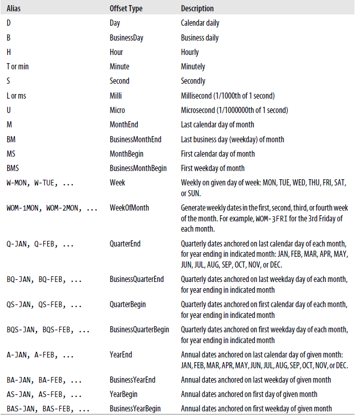
In [177]:Base Time Series Frequencies
Aggragate for duplicate Indices
In [157]: dates = pd.DatetimeIndex(['1/1/2000', '1/2/2000', '1/2/2000', '1/2/2000','1/3/2000','1/3/2000'])

In [158]: dates
Out[158]:
DatetimeIndex(['2000-01-01', '2000-01-02', '2000-01-02', '2000-01-02',
               '2000-01-03', '2000-01-03'],
              dtype='datetime64[ns]', freq=None)

In [159]: dup_ts = pd.Series(np.arange(6), index=dates)

In [160]: dup_ts
Out[160]:
2000-01-01    0
2000-01-02    1
2000-01-02    2
2000-01-02    3
2000-01-03    4
2000-01-03    5
dtype: int64

In [161]: dup_ts.index.is_unique
Out[161]: False

In [162]: dup_ts['2000-01-01']
Out[162]: 0

In [163]: dup_ts['2000-01-02']
Out[163]:
2000-01-02    1
2000-01-02    2
2000-01-02    3
dtype: int64

In [164]: dup_ts['2000-01-03']
Out[164]:
2000-01-03    4
2000-01-03    5
dtype: int64

In [165]:

In [165]: grouped = dup_ts.groupby(level=0)

In [166]: grouped.mean()
Out[166]:
2000-01-01    0.0
2000-01-02    2.0
2000-01-03    4.5
dtype: float64

In [167]: grouped.count()
Out[167]:
2000-01-01    1
2000-01-02    3
2000-01-03    2
dtype: int64

In [168]: grouped.sum()
Out[168]:
2000-01-01    0
2000-01-02    6
2000-01-03    9
dtype: int64

In [169]:
Group by month or weekday by passing a function that accesses those fields on the time series’s index.
In [90]: rng = pd.date_range('1/1/2000', periods=100, freq='D')
In [91]: ts = pd.Series(np.arange(100), index=rng)
In [92]: ts.groupby(lambda x: x.month).mean()
Out[92]:
1 15
2 45
3 75
4 95
dtype: int64
In [93]: ts.groupby(lambda x: x.month).sum()
Out[93]:
1 465
2 1305
3 2325
4 855
dtype: int64
In [94]: ts.groupby(lambda x: x.month).max()
Out[94]:
1 30
2 59
3 90
4 99
dtype: int64
In [95]: ts.groupby(lambda x: x.weekday).mean()
Out[95]:
0 47.5
1 48.5
2 49.5
3 50.5
4 51.5
5 49.0
6 50.0
dtype: float64
In [96]: ts.groupby(lambda x: x.weekday).sum()
Out[96]:
0 665
1 679
2 693
3 707
4 721
5 735
6 750
dtype: int64
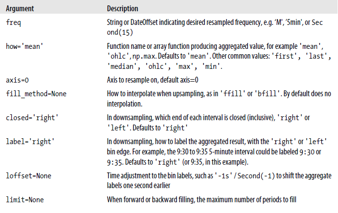
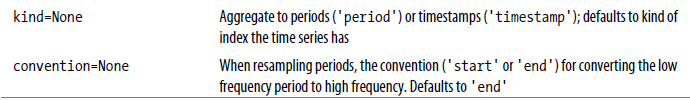
In [97]: Resample method arguments
Resampling and Frequency Conversion
In [50]: rng = pd.date_range('1/1/2000', periods=100, freq='D')

In [51]: ts = pd.Series(np.random.randn(len(rng)), index=rng)

In [52]: ts
Out[52]:
2000-01-01    0.030631
2000-01-02   -2.087034
2000-01-03    1.238687
2000-01-04   -1.297059
2000-01-05   -1.341296
2000-01-06   -0.353311
2000-01-07   -0.854693
2000-01-08    0.426789
                ...
2000-03-27    1.262705
2000-03-28   -0.646236
2000-03-29   -0.349658
2000-03-30   -1.093438
2000-03-31   -0.254758
2000-04-01    0.146417
2000-04-02    1.774502
2000-04-03   -0.712635
2000-04-04   -1.552352
2000-04-05    0.303172
2000-04-06   -0.023492
2000-04-07   -1.418930
2000-04-08    0.789877
2000-04-09    1.767594
Freq: D, Length: 100, dtype: float64

In [53]:

In [53]: ts.resample('M').mean()
Out[53]:
2000-01-31    0.003531
2000-02-29    0.030067
2000-03-31   -0.106783
2000-04-30    0.119350
Freq: M, dtype: float64

In [54]: ts.resample('M',kind='period').mean()
Out[54]:
2000-01    0.003531
2000-02    0.030067
2000-03   -0.106783
2000-04    0.119350
Freq: M, dtype: float64

In [55]:
Aggregate this data into five-minute chunks or bars by taking the sum of each group.
In [71]: rng = pd.date_range('1/1/2000', periods=24, freq='T')

In [72]: rng
Out[72]:
DatetimeIndex(['2000-01-01 00:00:00', '2000-01-01 00:01:00',
               '2000-01-01 00:02:00', '2000-01-01 00:03:00',
               '2000-01-01 00:04:00', '2000-01-01 00:05:00',
               '2000-01-01 00:06:00', '2000-01-01 00:07:00',
               '2000-01-01 00:08:00', '2000-01-01 00:09:00',
               '2000-01-01 00:10:00', '2000-01-01 00:11:00',
               '2000-01-01 00:12:00', '2000-01-01 00:13:00',
               '2000-01-01 00:14:00', '2000-01-01 00:15:00',
               '2000-01-01 00:16:00', '2000-01-01 00:17:00',
               '2000-01-01 00:18:00', '2000-01-01 00:19:00',
               '2000-01-01 00:20:00', '2000-01-01 00:21:00',
               '2000-01-01 00:22:00', '2000-01-01 00:23:00'],
              dtype='datetime64[ns]', freq='T')

In [73]: ts = pd.Series(np.arange(24), index=rng)

In [74]: ts
Out[74]:
2000-01-01 00:00:00     0
2000-01-01 00:01:00     1
2000-01-01 00:02:00     2
2000-01-01 00:03:00     3
2000-01-01 00:04:00     4
2000-01-01 00:05:00     5
2000-01-01 00:06:00     6
2000-01-01 00:07:00     7
2000-01-01 00:08:00     8
2000-01-01 00:09:00     9
2000-01-01 00:10:00    10
2000-01-01 00:11:00    11
2000-01-01 00:12:00    12
2000-01-01 00:13:00    13
2000-01-01 00:14:00    14
2000-01-01 00:15:00    15
2000-01-01 00:16:00    16
2000-01-01 00:17:00    17
2000-01-01 00:18:00    18
2000-01-01 00:19:00    19
2000-01-01 00:20:00    20
2000-01-01 00:21:00    21
2000-01-01 00:22:00    22
2000-01-01 00:23:00    23
Freq: T, dtype: int64

In [75]: ts.resample('5min').sum()
Out[75]:
2000-01-01 00:00:00    10
2000-01-01 00:05:00    35
2000-01-01 00:10:00    60
2000-01-01 00:15:00    85
2000-01-01 00:20:00    86
Freq: 5T, dtype: int64

In [76]: ts.resample('5min',closed='left').sum()
Out[76]:
2000-01-01 00:00:00    10
2000-01-01 00:05:00    35
2000-01-01 00:10:00    60
2000-01-01 00:15:00    85
2000-01-01 00:20:00    86
Freq: 5T, dtype: int64

In [77]:

In [77]: ts.resample('5min').max()
Out[77]:
2000-01-01 00:00:00     4
2000-01-01 00:05:00     9
2000-01-01 00:10:00    14
2000-01-01 00:15:00    19
2000-01-01 00:20:00    23
Freq: 5T, dtype: int64

In [78]:

In [78]: ts.resample('5min',closed='right').sum()
Out[78]:
1999-12-31 23:55:00     0
2000-01-01 00:00:00    15
2000-01-01 00:05:00    40
2000-01-01 00:10:00    65
2000-01-01 00:15:00    90
2000-01-01 00:20:00    66
Freq: 5T, dtype: int64

In [79]:

In [79]: ts.resample('5min',loffset='-1s').sum()
Out[79]:
1999-12-31 23:59:59    10
2000-01-01 00:04:59    35
2000-01-01 00:09:59    60
2000-01-01 00:14:59    85
2000-01-01 00:19:59    86
Freq: 5T, dtype: int64

In [80]:


# Open-High-Low-Close (OHLC) resampling
In [81]: ts.resample('5min').ohlc()
Out[81]:
                     open  high  low  close
2000-01-01 00:00:00     0     4    0      4
2000-01-01 00:05:00     5     9    5      9
2000-01-01 00:10:00    10    14   10     14
2000-01-01 00:15:00    15    19   15     19
2000-01-01 00:20:00    20    23   20     23

In [82]:
Resampling with Periods
In [118]: frame = pd.DataFrame(np.random.randn(24, 4),
     ...:     index=pd.period_range('1-2000', '12-2001', freq='M'),
     ...:     columns=['Beijing', 'Luoyang', 'New York', 'Tokyo'])

In [119]: frame
Out[119]:
          Beijing   Luoyang  New York     Tokyo
2000-01  1.120268 -1.120345 -1.154800  0.443861
2000-02  0.611443  0.200576 -1.163600 -1.137567
2000-03  0.658112  2.332235 -1.718285  1.589246
2000-04 -0.863050  1.890877  2.046202  0.410414
2000-05  0.710052 -0.041623  0.122719 -1.141112
2000-06  0.299393  1.227689  0.718627  1.004851
2000-07  1.287335 -0.179045 -0.476422  0.949235
2000-08 -2.140590  0.433699 -0.783202  1.073706
2000-09 -0.149710 -0.580780  0.755274  0.514259
2000-10  0.190940 -0.187451  1.710803 -1.631272
2000-11  0.419288  0.565235  0.470381  0.599020
2000-12  0.951111  0.464671 -0.854858 -0.009189
2001-01 -1.383493 -0.147035 -0.379006  0.472686
2001-02  1.803475 -1.628368 -0.896757 -0.508827
2001-03  0.575910 -0.528299  1.182473  0.159452
2001-04 -1.056161 -0.475357  0.861852  1.168667
2001-05 -1.316565  0.354719  1.354205 -0.369083
2001-06  0.497406 -1.799904 -0.512882 -0.092718
2001-07  0.896944 -1.276022  0.137365  0.087199
2001-08 -0.046908 -0.650024  0.958182 -0.048369
2001-09  0.085401  1.067235  0.541318  0.853376
2001-10  1.165047 -0.794425  1.137002  0.064595
2001-11 -0.438006  0.706564  1.464403  0.278069
2001-12 -0.094644  0.666789  0.220349 -0.386617

In [120]: frame[:5]
Out[120]:
          Beijing   Luoyang  New York     Tokyo
2000-01  1.120268 -1.120345 -1.154800  0.443861
2000-02  0.611443  0.200576 -1.163600 -1.137567
2000-03  0.658112  2.332235 -1.718285  1.589246
2000-04 -0.863050  1.890877  2.046202  0.410414
2000-05  0.710052 -0.041623  0.122719 -1.141112

In [121]: annual_frame = frame.resample('A-DEC').mean()

In [122]: annual_frame
Out[122]:
       Beijing   Luoyang  New York     Tokyo
2000  0.257883  0.417145 -0.027263  0.222121
2001  0.057367 -0.375344  0.505709  0.139869

In [123]:

In [123]: annual_frame_max = frame.resample('A-DEC').max()

In [124]: annual_frame_max
Out[124]:
       Beijing   Luoyang  New York     Tokyo
2000  1.287335  2.332235  2.046202  1.589246
2001  1.803475  1.067235  1.464403  1.168667

In [125]:
DataFrame
# 第一种定义pandas.DataFrame方式:直接导入numpy的数据
In [186]: df1 = pd.DataFrame(np.arange(12).reshape((3,4)))    # 定义pandas.DataFrame

In [187]: print(df1)
   0  1   2   3
0  0  1   2   3
1  4  5   6   7
2  8  9  10  11

In [188]:

In [178]: dates = pd.date_range('20160101',periods=6)

In [179]: print(dates)
DatetimeIndex(['2016-01-01', '2016-01-02', '2016-01-03', '2016-01-04',
               '2016-01-05', '2016-01-06'],
              dtype='datetime64[ns]', freq='D')

In [180]:

# 定义pandas.DataFrame,并指定列名和行名
In [184]: df = pd.DataFrame(np.random.randn(6,4),index=dates,columns=['a','b','c','d'])

In [185]: print(df)
                   a         b         c         d
2016-01-01  1.193589  0.165348  1.598806 -0.478980
2016-01-02  1.188886 -1.232185 -0.633066  0.594805
2016-01-03  2.707996 -0.116420  1.622761  0.399708
2016-01-04  0.416469  1.593061 -0.044390 -0.031153
2016-01-05 -0.637080  1.680110  1.371026  0.821549
2016-01-06 -0.079359  1.421577  0.042537  1.058749

In [186]:


# 第二种定义pandas.DataFrame方式:把参数当做字典传入DataFrame
In [188]: df2 = pd.DataFrame({'A' : 1.,
     ...:                     'B' : pd.Timestamp('20130102'),
     ...:                     'C' : pd.Series(1,index=list(range(4)),dtype='float32'),
     ...:                     'D' : np.array([3] * 4,dtype='int32'),
     ...:                     'E' : pd.Categorical(["test","train","test","train"]),
     ...:                     'F' : 'foo'})

In [189]: print(df2)
     A          B    C  D      E    F
0  1.0 2013-01-02  1.0  3   test  foo
1  1.0 2013-01-02  1.0  3  train  foo
2  1.0 2013-01-02  1.0  3   test  foo
3  1.0 2013-01-02  1.0  3  train  foo

In [190]:
In [190]: print(df2.dtypes)                      # 查看DataFrame内容的类型
A           float64
B    datetime64[ns]
C           float32
D             int32
E          category
F            object
dtype: object

In [191]:
In [191]: print(df2.index)                       # 打印DataFrame列的名字
Int64Index([0, 1, 2, 3], dtype='int64')

In [192]:
In [192]: print(df2.columns)                     # 打印DataFrame行的名字
Index([u'A', u'B', u'C', u'D', u'E', u'F'], dtype='object')

In [193]:

In [194]: print(df2.values)                      # 打印DataFrame的内容
[[1.0 Timestamp('2013-01-02 00:00:00') 1.0 3 'test' 'foo']
 [1.0 Timestamp('2013-01-02 00:00:00') 1.0 3 'train' 'foo']
 [1.0 Timestamp('2013-01-02 00:00:00') 1.0 3 'test' 'foo']
 [1.0 Timestamp('2013-01-02 00:00:00') 1.0 3 'train' 'foo']]

In [195]:


In [196]: print(df2)
     A          B    C  D      E    F
0  1.0 2013-01-02  1.0  3   test  foo
1  1.0 2013-01-02  1.0  3  train  foo
2  1.0 2013-01-02  1.0  3   test  foo
3  1.0 2013-01-02  1.0  3  train  foo

In [197]:

In [197]: print(df2.describe())                  # 打印出DataFrame的数学运算的相关数据
         A    C    D
count  4.0  4.0  4.0
mean   1.0  1.0  3.0
std    0.0  0.0  0.0
min    1.0  1.0  3.0
25%    1.0  1.0  3.0
50%    1.0  1.0  3.0
75%    1.0  1.0  3.0
max    1.0  1.0  3.0

In [198]:


In [200]: print(df2.T)                           # 把DataFrame进行transport,即转置
                     0                    1                    2                    3
A                    1                    1                    1                    1
B  2013-01-02 00:00:00  2013-01-02 00:00:00  2013-01-02 00:00:00  2013-01-02 00:00:00
C                    1                    1                    1                    1
D                    3                    3                    3                    3
E                 test                train                 test                train
F                  foo                  foo                  foo                  foo

In [201]:


# 对DataFrame排序
In [203]: print(df2)
     A          B    C  D      E    F
0  1.0 2013-01-02  1.0  3   test  foo
1  1.0 2013-01-02  1.0  3  train  foo
2  1.0 2013-01-02  1.0  3   test  foo
3  1.0 2013-01-02  1.0  3  train  foo

In [204]: df2.sort_index(axis=1, ascending=False)   # 按照index(列名)排序
Out[204]:
     F      E  D    C          B    A
0  foo   test  3  1.0 2013-01-02  1.0
1  foo  train  3  1.0 2013-01-02  1.0
2  foo   test  3  1.0 2013-01-02  1.0
3  foo  train  3  1.0 2013-01-02  1.0

In [205]:
In [205]: df2.sort_index(axis=0, ascending=False)   # 按照行名排序
Out[205]:
     A          B    C  D      E    F
3  1.0 2013-01-02  1.0  3  train  foo
2  1.0 2013-01-02  1.0  3   test  foo
1  1.0 2013-01-02  1.0  3  train  foo
0  1.0 2013-01-02  1.0  3   test  foo

In [206]:


In [207]: df2.sort_values(by='E')                   # 指定value进行排序
Out[207]:
     A          B    C  D      E    F
0  1.0 2013-01-02  1.0  3   test  foo
2  1.0 2013-01-02  1.0  3   test  foo
1  1.0 2013-01-02  1.0  3  train  foo
3  1.0 2013-01-02  1.0  3  train  foo

In [208]:
Pandas筛选数据
In [212]: dates = pd.date_range('20160101',periods=6)

In [213]: df = pd.DataFrame(np.arange(24).reshape(6,4),index=dates,columns=['A','B','C','D'])

In [214]: print(df)
             A   B   C   D
2016-01-01   0   1   2   3
2016-01-02   4   5   6   7
2016-01-03   8   9  10  11
2016-01-04  12  13  14  15
2016-01-05  16  17  18  19
2016-01-06  20  21  22  23

In [215]:

In [215]: print(df['A'])            # 选取指定列
2016-01-01     0
2016-01-02     4
2016-01-03     8
2016-01-04    12
2016-01-05    16
2016-01-06    20
Freq: D, Name: A, dtype: int64

In [216]: print(df.A)               # 等价于 df['A']
2016-01-01     0
2016-01-02     4
2016-01-03     8
2016-01-04    12
2016-01-05    16
2016-01-06    20
Freq: D, Name: A, dtype: int64

In [217]:

In [217]: print(df[0:3])            # 切片方式选取某些行
            A  B   C   D
2016-01-01  0  1   2   3
2016-01-02  4  5   6   7
2016-01-03  8  9  10  11

In [218]: print(df['2016-01-01':'2016-01-03'])   # 等价于 df[0:3]
            A  B   C   D
2016-01-01  0  1   2   3
2016-01-02  4  5   6   7
2016-01-03  8  9  10  11

In [219]:


# select by label : loc
In [220]: print(df.loc['2016-01-02'])
A    4
B    5
C    6
D    7
Name: 2016-01-02 00:00:00, dtype: int64

In [221]:
In [221]: print(df.loc['2016-01-02']['B'])
5

In [222]:

In [227]: print(df.loc[:,['A','B']])
             A   B
2016-01-01   0   1
2016-01-02   4   5
2016-01-03   8   9
2016-01-04  12  13
2016-01-05  16  17
2016-01-06  20  21

In [228]:
In [228]: print(df.loc['2016-01-03',['A','B']])
A    8
B    9
Name: 2016-01-03 00:00:00, dtype: int64

In [229]:
In [232]: print(df.loc['2016-01-03':'2016-01-05',['A','B']])
             A   B
2016-01-03   8   9
2016-01-04  12  13
2016-01-05  16  17

In [233]:


# select by position : iloc
In [235]: print(df)
             A   B   C   D
2016-01-01   0   1   2   3
2016-01-02   4   5   6   7
2016-01-03   8   9  10  11
2016-01-04  12  13  14  15
2016-01-05  16  17  18  19
2016-01-06  20  21  22  23

In [236]: print(df.iloc[3])
A    12
B    13
C    14
D    15
Name: 2016-01-04 00:00:00, dtype: int64

In [237]: print(df.iloc[3,1])
13

In [238]:

In [238]: print(df.iloc[3:5,1:3])
             B   C
2016-01-04  13  14
2016-01-05  17  18

In [239]:

In [240]: print(df.iloc[[1,3,5],1:3])
             B   C
2016-01-02   5   6
2016-01-04  13  14
2016-01-06  21  22

In [241]:


# mixed selection : ix
In [243]: print(df.ix[:3,['A','C']])
/usr/local/anaconda2/bin/ipython2:1: DeprecationWarning:
.ix is deprecated. Please use
.loc for label based indexing or
.iloc for positional indexing

See the documentation here:
http://pandas.pydata.org/pandas-docs/stable/indexing.html#ix-indexer-is-deprecated
  #!/usr/local/anaconda2/bin/python
            A   C
2016-01-01  0   2
2016-01-02  4   6
2016-01-03  8  10

In [244]:


# Boolean indexing
In [9]: print(df[df.A>8])
             A   B   C   D
2016-01-04  12  13  14  15
2016-01-05  16  17  18  19
2016-01-06  20  21  22  23

In [10]:
df.head(n) # 返回DataFrame前n行
df.tail(n) # 返回DateFrame后n行Pandas设置值
# 给DataFrame设置值
In [1]: import numpy as np

In [2]: import pandas as pd

In [3]: dates = pd.date_range('20160101',periods=6)

In [4]: df = pd.DataFrame(np.arange(24).reshape(6,4),index=dates,columns=['A','B','C','D'])

In [5]: print(df)
             A   B   C   D
2016-01-01   0   1   2   3
2016-01-02   4   5   6   7
2016-01-03   8   9  10  11
2016-01-04  12  13  14  15
2016-01-05  16  17  18  19
2016-01-06  20  21  22  23

In [6]:
In [7]: df.iloc[2,2] = 99

In [10]: df.loc['2016-01-02','B'] = 100

In [11]: print(df)
             A    B   C   D
2016-01-01   0    1   2   3
2016-01-02   4  100   6   7
2016-01-03   8    9  99  11
2016-01-04  12   13  14  15
2016-01-05  16   17  18  19
2016-01-06  20   21  22  23

In [12]:


In [17]: print(df)
             A   B   C   D
2016-01-01   0   1   2   3
2016-01-02   4   5   6   7
2016-01-03   8   9  10  11
2016-01-04  12  13  14  15
2016-01-05  16  17  18  19
2016-01-06  20  21  22  23

In [18]: df.A[df.A>4] = 0

In [19]: print(df)
            A   B   C   D
2016-01-01  0   1   2   3
2016-01-02  4   5   6   7
2016-01-03  0   9  10  11
2016-01-04  0  13  14  15
2016-01-05  0  17  18  19
2016-01-06  0  21  22  23

In [20]:


In [21]: print(df)
             A   B   C   D
2016-01-01   0   1   2   3
2016-01-02   4   5   6   7
2016-01-03   8   9  10  11
2016-01-04  12  13  14  15
2016-01-05  16  17  18  19
2016-01-06  20  21  22  23

In [22]: df[df.A>4] = 0

In [23]: print(df)
            A  B  C  D
2016-01-01  0  1  2  3
2016-01-02  4  5  6  7
2016-01-03  0  0  0  0
2016-01-04  0  0  0  0
2016-01-05  0  0  0  0
2016-01-06  0  0  0  0

In [24]:


In [30]: df['F'] = np.nan        # 增加一列,赋值为NaN

In [31]: print(df)
             A   B   C   D   F
2016-01-01   0   1   2   3 NaN
2016-01-02   4   5   6   7 NaN
2016-01-03   8   9  10  11 NaN
2016-01-04  12  13  14  15 NaN
2016-01-05  16  17  18  19 NaN
2016-01-06  20  21  22  23 NaN

In [32]:
                                 # 增加一列,需要制定行名
In [46]: df['F'] = pd.Series([1,2,3,4,5,6], index=pd.date_range('20160101',periods=6))

In [47]: print(df)
             A   B   C   D   E  F
2016-01-01   0   1   2   3 NaN  1
2016-01-02   4   5   6   7 NaN  2
2016-01-03   8   9  10  11 NaN  3
2016-01-04  12  13  14  15 NaN  4
2016-01-05  16  17  18  19 NaN  5
2016-01-06  20  21  22  23 NaN  6

In [48]:
Pandas删除DataFrame数据
In [1]: import numpy as np

In [2]: import pandas as pd

In [3]: values = np.arange(12).reshape((3,4))

In [4]: print(values)
[[ 0  1  2  3]
 [ 4  5  6  7]
 [ 8  9 10 11]]

In [5]:
In [8]: df = pd.DataFrame(values,index=['row1','row2','row3'],columns=['A','B','C','D'])

In [9]: print(df)
      A  B   C   D
row1  0  1   2   3
row2  4  5   6   7
row3  8  9  10  11

In [10]:
In [10]: print(df.shape)
(3, 4)

In [11]:
In [11]: df.drop(columns='A',axis=1)
Out[11]:
      B   C   D
row1  1   2   3
row2  5   6   7
row3  9  10  11

In [12]: df.drop(columns=['A','C'],axis=1)
Out[12]:
      B   D
row1  1   3
row2  5   7
row3  9  11

In [13]:

In [13]: df.drop(index='row2',axis=0)
Out[13]:
      A  B   C   D
row1  0  1   2   3
row3  8  9  10  11

In [14]: df.drop(index=['row2','row3'],axis=0)
Out[14]:
      A  B  C  D
row1  0  1  2  3

In [15]:
如果index用的是 “pd.date_range('20160101',periods=6)”
In [43]: print(df)
                   a         b         c         d
2016-01-01  1.273748  0.949407 -0.446053 -0.126789
2016-01-02 -0.770801  1.641150  0.840216 -0.991219
2016-01-03 -0.164625 -1.459954  1.214388  0.281621
2016-01-04  1.863281  1.163653  0.319549 -1.545655
2016-01-05  0.452804  0.203472 -1.232536  0.681963
2016-01-06  0.171324  0.353359  1.674004 -2.026071

In [44]: print(df.index)
DatetimeIndex(['2016-01-01', '2016-01-02', '2016-01-03', '2016-01-04',
               '2016-01-05', '2016-01-06'],
              dtype='datetime64[ns]', freq='D')

In [45]:

In [45]: df.drop(index=pd.datetime(2016,1,4),axis=0)
Out[45]:
                   a         b         c         d
2016-01-01  1.273748  0.949407 -0.446053 -0.126789
2016-01-02 -0.770801  1.641150  0.840216 -0.991219
2016-01-03 -0.164625 -1.459954  1.214388  0.281621
2016-01-05  0.452804  0.203472 -1.232536  0.681963
2016-01-06  0.171324  0.353359  1.674004 -2.026071

In [46]: df.drop(index=[pd.datetime(2016,1,2),pd.datetime(2016,1,5)],axis=0)
Out[46]:
                   a         b         c         d
2016-01-01  1.273748  0.949407 -0.446053 -0.126789
2016-01-03 -0.164625 -1.459954  1.214388  0.281621
2016-01-04  1.863281  1.163653  0.319549 -1.545655
2016-01-06  0.171324  0.353359  1.674004 -2.026071

In [47]:
Pandas处理丢失的数据
# 处理丢失数据

In [7]: print(df)
             A   B   C   D
2016-01-01   0   1   2   3
2016-01-02   4   5   6   7
2016-01-03   8   9  10  11
2016-01-04  12  13  14  15
2016-01-05  16  17  18  19
2016-01-06  20  21  22  23

In [8]: df.iloc[0,1] = np.nan

In [9]: df.iloc[1,2] = np.nan

In [10]: print(df)
             A     B     C   D
2016-01-01   0   NaN   2.0   3
2016-01-02   4   5.0   NaN   7
2016-01-03   8   9.0  10.0  11
2016-01-04  12  13.0  14.0  15
2016-01-05  16  17.0  18.0  19
2016-01-06  20  21.0  22.0  23

In [11]: print(df.dropna(axis=1,how='any'))  # 删除NaN数据所在行,how = {'any','all'}
             A   D
2016-01-01   0   3
2016-01-02   4   7
2016-01-03   8  11
2016-01-04  12  15
2016-01-05  16  19
2016-01-06  20  23

In [12]: print(df.dropna(axis=0,how='any'))  # 删除NaN数据所在行,how = {'any','all'}
             A     B     C   D
2016-01-03   8   9.0  10.0  11
2016-01-04  12  13.0  14.0  15
2016-01-05  16  17.0  18.0  19
2016-01-06  20  21.0  22.0  23

In [13]:
In [13]: print(df.dropna(axis=0,how='all'))
             A     B     C   D
2016-01-01   0   NaN   2.0   3
2016-01-02   4   5.0   NaN   7
2016-01-03   8   9.0  10.0  11
2016-01-04  12  13.0  14.0  15
2016-01-05  16  17.0  18.0  19
2016-01-06  20  21.0  22.0  23

In [14]:
In [14]: print(df.dropna(axis=1,how='all'))
             A     B     C   D
2016-01-01   0   NaN   2.0   3
2016-01-02   4   5.0   NaN   7
2016-01-03   8   9.0  10.0  11
2016-01-04  12  13.0  14.0  15
2016-01-05  16  17.0  18.0  19
2016-01-06  20  21.0  22.0  23

In [15]:


In [15]: df.fillna(value=0)                # 把NaN填充为制定数值
Out[15]:
             A     B     C   D
2016-01-01   0   0.0   2.0   3
2016-01-02   4   5.0   0.0   7
2016-01-03   8   9.0  10.0  11
2016-01-04  12  13.0  14.0  15
2016-01-05  16  17.0  18.0  19
2016-01-06  20  21.0  22.0  23

In [16]:


In [19]: print(df.isnull())                # 把数值为NaN的位置标识出来
                A      B      C      D
2016-01-01  False   True  False  False
2016-01-02  False  False   True  False
2016-01-03  False  False  False  False
2016-01-04  False  False  False  False
2016-01-05  False  False  False  False
2016-01-06  False  False  False  False

In [20]:


In [22]: print(np.any(df.isnull()) == True)   # 检查DataFrame是否含有NaN值
True

In [23]:
Pandas导入导出示例
In [33]: import pandas as pd
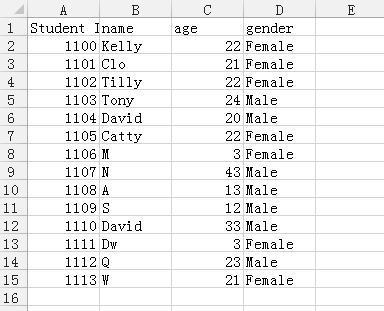
In [34]: data = pd.read_csv('student.csv')
In [35]: print(data)
Student ID name age gender
0 1100 Kelly 22 Female
1 1101 Clo 21 Female
2 1102 Tilly 22 Female
3 1103 Tony 24 Male
4 1104 David 20 Male
5 1105 Catty 22 Female
6 1106 M 3 Female
7 1107 N 43 Male
8 1108 A 13 Male
9 1109 S 12 Male
10 1110 David 33 Male
11 1111 Dw 3 Female
12 1112 Q 23 Male
13 1113 W 21 Female
In [36]: print(type(data))
<class 'pandas.core.frame.DataFrame'>
In [37]: data.to_pickle('student.pickle')
In [38]: data.to_json('student.json')
In [39]:更多IO Tools参考:官方介绍
Pandas concat合并
# pandas 合并

# concatenating
In [40]: import numpy as np

In [41]: import pandas as pd

In [42]: df1 = pd.DataFrame(np.ones((3,4))*0, columns=['a','b','c','d'])

In [43]: df2 = pd.DataFrame(np.ones((3,4))*1, columns=['a','b','c','d'])

In [44]: df3 = pd.DataFrame(np.ones((3,4))*2, columns=['a','b','c','d'])

In [45]: print(df1)
     a    b    c    d
0  0.0  0.0  0.0  0.0
1  0.0  0.0  0.0  0.0
2  0.0  0.0  0.0  0.0

In [46]: print(df2)
     a    b    c    d
0  1.0  1.0  1.0  1.0
1  1.0  1.0  1.0  1.0
2  1.0  1.0  1.0  1.0

In [47]: print(df3)
     a    b    c    d
0  2.0  2.0  2.0  2.0
1  2.0  2.0  2.0  2.0
2  2.0  2.0  2.0  2.0

In [48]: result = pd.concat([df1,df2,df3],axis=0)   # vertical 垂直合并

In [49]: print(result)
     a    b    c    d
0  0.0  0.0  0.0  0.0
1  0.0  0.0  0.0  0.0
2  0.0  0.0  0.0  0.0
0  1.0  1.0  1.0  1.0
1  1.0  1.0  1.0  1.0
2  1.0  1.0  1.0  1.0
0  2.0  2.0  2.0  2.0
1  2.0  2.0  2.0  2.0
2  2.0  2.0  2.0  2.0

In [50]:
In [50]: result = pd.concat([df1,df2,df3],axis=0,ignore_index=True)  # 序号重新排列

In [51]: print(result)
     a    b    c    d
0  0.0  0.0  0.0  0.0
1  0.0  0.0  0.0  0.0
2  0.0  0.0  0.0  0.0
3  1.0  1.0  1.0  1.0
4  1.0  1.0  1.0  1.0
5  1.0  1.0  1.0  1.0
6  2.0  2.0  2.0  2.0
7  2.0  2.0  2.0  2.0
8  2.0  2.0  2.0  2.0

In [52]:


# join合并   ['inner','outer']
In [63]: df1 = pd.DataFrame(np.ones((3,4))*0, columns=['a','b','c','d'],index=[1,2,3])

In [64]: df2 = pd.DataFrame(np.ones((3,4))*1, columns=['b','c','d','e'],index=[2,3,4])

In [65]: print(df1)
     a    b    c    d
1  0.0  0.0  0.0  0.0
2  0.0  0.0  0.0  0.0
3  0.0  0.0  0.0  0.0

In [66]: print(df2)
     b    c    d    e
2  1.0  1.0  1.0  1.0
3  1.0  1.0  1.0  1.0
4  1.0  1.0  1.0  1.0

In [67]:
In [67]: result = pd.concat([df1,df2])     # 即 pd.concat([df1,df2],join='outer') , 默认就是outer模式
/usr/local/anaconda2/bin/ipython2:1: FutureWarning: Sorting because non-concatenation axis is not aligned. A future version
of pandas will change to not sort by default.

To accept the future behavior, pass 'sort=True'.

To retain the current behavior and silence the warning, pass sort=False

  #!/usr/local/anaconda2/bin/python

In [68]:

In [68]: print(result)
     a    b    c    d    e
1  0.0  0.0  0.0  0.0  NaN
2  0.0  0.0  0.0  0.0  NaN
3  0.0  0.0  0.0  0.0  NaN
2  NaN  1.0  1.0  1.0  1.0
3  NaN  1.0  1.0  1.0  1.0
4  NaN  1.0  1.0  1.0  1.0

In [69]:

In [70]: result = pd.concat([df1,df2],join='inner')  # inner模式

In [71]: print(result)
     b    c    d
1  0.0  0.0  0.0
2  0.0  0.0  0.0
3  0.0  0.0  0.0
2  1.0  1.0  1.0
3  1.0  1.0  1.0
4  1.0  1.0  1.0

In [72]:
In [72]: result = pd.concat([df1,df2],join='inner',ignore_index=True)

In [73]: print(result)
     b    c    d
0  0.0  0.0  0.0
1  0.0  0.0  0.0
2  0.0  0.0  0.0
3  1.0  1.0  1.0
4  1.0  1.0  1.0
5  1.0  1.0  1.0

In [74]:


# join_axes合并
In [78]: res = pd.concat([df1, df2], axis=1)

In [79]: print(res)
     a    b    c    d    b    c    d    e
1  0.0  0.0  0.0  0.0  NaN  NaN  NaN  NaN
2  0.0  0.0  0.0  0.0  1.0  1.0  1.0  1.0
3  0.0  0.0  0.0  0.0  1.0  1.0  1.0  1.0
4  NaN  NaN  NaN  NaN  1.0  1.0  1.0  1.0

In [80]:
In [74]: df1 = pd.DataFrame(np.ones((3,4))*0, columns=['a','b','c','d'],index=[1,2,3])

In [75]: df2 = pd.DataFrame(np.ones((3,4))*1, columns=['b','c','d','e'],index=[2,3,4])

In [76]: res = pd.concat([df1, df2], axis=1, join_axes=[df1.index])

In [77]: print(res)
     a    b    c    d    b    c    d    e
1  0.0  0.0  0.0  0.0  NaN  NaN  NaN  NaN
2  0.0  0.0  0.0  0.0  1.0  1.0  1.0  1.0
3  0.0  0.0  0.0  0.0  1.0  1.0  1.0  1.0

In [78]:
In [80]: res = pd.concat([df1, df2], axis=1, join_axes=[df2.index])

In [81]: print(res)
     a    b    c    d    b    c    d    e
2  0.0  0.0  0.0  0.0  1.0  1.0  1.0  1.0
3  0.0  0.0  0.0  0.0  1.0  1.0  1.0  1.0
4  NaN  NaN  NaN  NaN  1.0  1.0  1.0  1.0

In [82]:


# append合并

In [87]: df1 = pd.DataFrame(np.ones((3,4))*0, columns=['a','b','c','d'])

In [88]: df2 = pd.DataFrame(np.ones((3,4))*1, columns=['a','b','c','d'])

In [89]: df1.append(df2,ignore_index=True)
Out[89]:
     a    b    c    d
0  0.0  0.0  0.0  0.0
1  0.0  0.0  0.0  0.0
2  0.0  0.0  0.0  0.0
3  1.0  1.0  1.0  1.0
4  1.0  1.0  1.0  1.0
5  1.0  1.0  1.0  1.0

In [90]: df3 = pd.DataFrame(np.ones((3,4))*1, columns=['a','b','c','d'])

In [91]: df1.append([df2,df3],ignore_index=True)
Out[91]:
     a    b    c    d
0  0.0  0.0  0.0  0.0
1  0.0  0.0  0.0  0.0
2  0.0  0.0  0.0  0.0
3  1.0  1.0  1.0  1.0
4  1.0  1.0  1.0  1.0
5  1.0  1.0  1.0  1.0
6  1.0  1.0  1.0  1.0
7  1.0  1.0  1.0  1.0
8  1.0  1.0  1.0  1.0

In [92]:


# 添加一行数据到DataFrame
In [92]: df1 = pd.DataFrame(np.ones((3,4))*0, columns=['a','b','c','d'])

In [93]: s1 = pd.Series([1,2,3,4], index=['a','b','c','d'])

In [94]: res = df1.append(s1,ignore_index=True)

In [95]: print(res)
     a    b    c    d
0  0.0  0.0  0.0  0.0
1  0.0  0.0  0.0  0.0
2  0.0  0.0  0.0  0.0
3  1.0  2.0  3.0  4.0

In [96]:
Pandas merge合并
# merge合并
In [99]: import pandas as pd

In [100]: left = pd.DataFrame({'key': ['K0', 'K1', 'K2', 'K3'],
     ...:                      'A': ['A0', 'A1', 'A2', 'A3'],
     ...:                      'B': ['B0', 'B1', 'B2', 'B3']})

In [101]: right = pd.DataFrame({'key': ['K0', 'K1', 'K2', 'K3'],
     ...:                       'C': ['C0', 'C1', 'C2', 'C3'],
     ...:                       'D': ['D0', 'D1', 'D2', 'D3']})

In [102]:

In [102]: print(left)
    A   B key
0  A0  B0  K0
1  A1  B1  K1
2  A2  B2  K2
3  A3  B3  K3

In [103]: print(right)
    C   D key
0  C0  D0  K0
1  C1  D1  K1
2  C2  D2  K2
3  C3  D3  K3

In [104]:
In [104]: res = pd.merge(left,right,on='key')

In [105]: print(res)
    A   B key   C   D
0  A0  B0  K0  C0  D0
1  A1  B1  K1  C1  D1
2  A2  B2  K2  C2  D2
3  A3  B3  K3  C3  D3

In [106]:


# consider two keys
In [106]: left = pd.DataFrame({'key1': ['K0', 'K0', 'K1', 'K2'],
     ...:                       'key2': ['K0', 'K1', 'K0', 'K1'],
     ...:                       'A': ['A0', 'A1', 'A2', 'A3'],
     ...:                       'B': ['B0', 'B1', 'B2', 'B3']})

In [107]: right = pd.DataFrame({'key1': ['K0', 'K1', 'K1', 'K2'],
     ...:                        'key2': ['K0', 'K0', 'K0', 'K0'],
     ...:                        'C': ['C0', 'C1', 'C2', 'C3'],
     ...:                        'D': ['D0', 'D1', 'D2', 'D3']})

In [108]: print(left)
    A   B key1 key2
0  A0  B0   K0   K0
1  A1  B1   K0   K1
2  A2  B2   K1   K0
3  A3  B3   K2   K1

In [109]: print(right)
    C   D key1 key2
0  C0  D0   K0   K0
1  C1  D1   K1   K0
2  C2  D2   K1   K0
3  C3  D3   K2   K0

In [110]: res = pd.merge(left,right,on=['key1','key2'])

In [111]: print(res)
    A   B key1 key2   C   D
0  A0  B0   K0   K0  C0  D0
1  A2  B2   K1   K0  C1  D1
2  A2  B2   K1   K0  C2  D2


# how={'left','right','inner','outer'}
In [112]: res = pd.merge(left,right,on=['key1','key2'],how='inner')  # 默认就是inner模式

In [113]: print(res)
    A   B key1 key2   C   D
0  A0  B0   K0   K0  C0  D0
1  A2  B2   K1   K0  C1  D1
2  A2  B2   K1   K0  C2  D2

In [114]: res = pd.merge(left,right,on=['key1','key2'],how='outer')

In [115]: print(res)
     A    B key1 key2    C    D
0   A0   B0   K0   K0   C0   D0
1   A1   B1   K0   K1  NaN  NaN
2   A2   B2   K1   K0   C1   D1
3   A2   B2   K1   K0   C2   D2
4   A3   B3   K2   K1  NaN  NaN
5  NaN  NaN   K2   K0   C3   D3

In [116]:
In [116]: res = pd.merge(left,right,on=['key1','key2'],how='left')

In [117]: print(res)
    A   B key1 key2    C    D
0  A0  B0   K0   K0   C0   D0
1  A1  B1   K0   K1  NaN  NaN
2  A2  B2   K1   K0   C1   D1
3  A2  B2   K1   K0   C2   D2
4  A3  B3   K2   K1  NaN  NaN

In [118]: res = pd.merge(left,right,on=['key1','key2'],how='right')

In [119]: print(res)
     A    B key1 key2   C   D
0   A0   B0   K0   K0  C0  D0
1   A2   B2   K1   K0  C1  D1
2   A2   B2   K1   K0  C2  D2
3  NaN  NaN   K2   K0  C3  D3

In [120]:


# indicator
In [121]: df1 = pd.DataFrame({'col1':[0,1], 'col_left':['a','b']})

In [122]: df2 = pd.DataFrame({'col1':[1,2,2],'col_right':[2,2,2]})

In [123]: print(df1)
   col1 col_left
0     0        a
1     1        b

In [124]: print(df2)
   col1  col_right
0     1          2
1     2          2
2     2          2

In [125]: res = pd.merge(df1, df2, on='col1', how='outer', indicator=True) # 给一个提示

In [126]: print(res)
   col1 col_left  col_right      _merge
0     0        a        NaN   left_only
1     1        b        2.0        both
2     2      NaN        2.0  right_only
3     2      NaN        2.0  right_only

In [127]:
In [129]: res = pd.merge(df1, df2, on='col1', how='outer', indicator='indicator_column') # 指定提示的列名

In [130]: print(res)
   col1 col_left  col_right indicator_column
0     0        a        NaN        left_only
1     1        b        2.0             both
2     2      NaN        2.0       right_only
3     2      NaN        2.0       right_only

In [131]:
In [127]: res = pd.merge(df1, df2, on='col1', how='outer', indicator=False)

In [128]: print(res)
   col1 col_left  col_right
0     0        a        NaN
1     1        b        2.0
2     2      NaN        2.0
3     2      NaN        2.0

In [129]:


In [131]: left = pd.DataFrame({'A': ['A0', 'A1', 'A2'],
     ...:                      'B': ['B0', 'B1', 'B2']},
     ...:                      index=['K0', 'K1', 'K2'])

In [132]: right = pd.DataFrame({'C': ['C0', 'C2', 'C3'],
     ...:                       'D': ['D0', 'D2', 'D3']},
     ...:                      index=['K0', 'K2', 'K3'])

In [133]: print(left)
     A   B
K0  A0  B0
K1  A1  B1
K2  A2  B2

In [134]: print(right)
     C   D
K0  C0  D0
K2  C2  D2
K3  C3  D3

In [135]: res = pd.merge(left, right, left_index=True, right_index=True, how='outer')

In [136]: print(res)
      A    B    C    D
K0   A0   B0   C0   D0
K1   A1   B1  NaN  NaN
K2   A2   B2   C2   D2
K3  NaN  NaN   C3   D3

In [137]: res = pd.merge(left, right, left_index=True, right_index=True, how='inner')

In [138]: print(res)
     A   B   C   D
K0  A0  B0  C0  D0
K2  A2  B2  C2  D2

In [139]:


# handle overlapping
In [139]: boys = pd.DataFrame({'k': ['K0', 'K1', 'K2'], 'age': [1, 2, 3]})

In [140]: girls = pd.DataFrame({'k': ['K0', 'K0', 'K3'], 'age': [4, 5, 6]})

In [141]: print(boys)
   age   k
0    1  K0
1    2  K1
2    3  K2

In [142]: print(girls)
   age   k
0    4  K0
1    5  K0
2    6  K3

In [143]: res = pd.merge(boys, girls, on='k', suffixes=['_boy', '_girl'], how='inner')

In [144]: print(res)
   age_boy   k  age_girl
0        1  K0         4
1        1  K0         5

In [145]: res = pd.merge(boys, girls, on='k', suffixes=['_boy', '_girl'], how='outer')

In [146]: print(res)
   age_boy   k  age_girl
0      1.0  K0       4.0
1      1.0  K0       5.0
2      2.0  K1       NaN
3      3.0  K2       NaN
4      NaN  K3       6.0

In [147]:
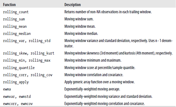
Pandas Moving Window Functions
Pandas plot可视化
#!/usr/bin/python2.7

import numpy as np
import pandas as pd
import matplotlib.pyplot as plt

# Series
data = pd.Series(np.random.randn(1000),index=np.arange(1000))

data = data.cumsum()


data.plot()
plt.show()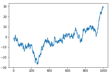
#!/usr/bin/python2.7
import numpy as np
import pandas as pd
import matplotlib.pyplot as plt
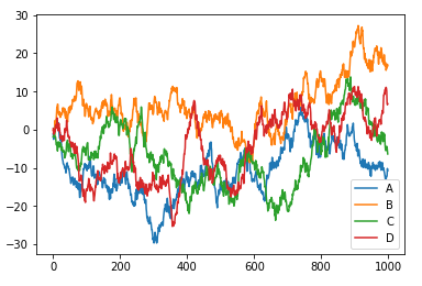
# DataFrame
data = pd.DataFrame(np.random.randn(1000,4),\
index=np.arange(1000), \
columns=list("ABCD"))
data = data.cumsum()
# print(data.head(6))
data.plot()
plt.show()
#!/usr/bin/python2.7
import numpy as np
import pandas as pd
import matplotlib.pyplot as plt
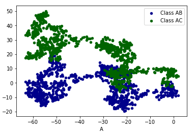
# DataFrame
data = pd.DataFrame(np.random.randn(1000,4),\
index=np.arange(1000), \
columns=list("ABCD"))
data = data.cumsum()
# print(data.head(6))
# plot method:
# 'bar','hist','box','kde','aera','scatter','pie','hexbin'...
ax = data.plot.scatter(x='A',y='B',color='DarkBlue',label='Class AB')
data.plot.scatter(x='A',y='C',color='DarkGreen',label='Class AC',ax=ax)
plt.show()
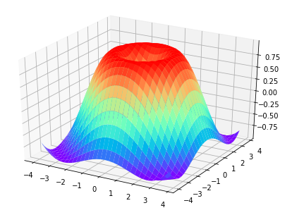
补充:Matplotlib 3D图像
#!/usr/bin/python2.7

import numpy as np
import matplotlib.pyplot as plt
from mpl_toolkits.mplot3d import Axes3D

fig = plt.figure()
ax = Axes3D(fig)

# X,Y value
X = np.arange(-4,4,0.25)
Y = np.arange(-4,4,0.25)
X,Y = np.meshgrid(X,Y)
R = np.sqrt(X**2+Y**2)

# height value
Z = np.sin(R)

ax.plot_surface(X,Y,Z,rstride=1,cstride=1,cmap=plt.get_cmap('rainbow'))

plt.show()
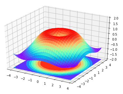
#!/usr/bin/python2.7

import numpy as np
import matplotlib.pyplot as plt
from mpl_toolkits.mplot3d import Axes3D

fig = plt.figure()
ax = Axes3D(fig)

# X,Y value
X = np.arange(-4,4,0.25)
Y = np.arange(-4,4,0.25)
X,Y = np.meshgrid(X,Y)
R = np.sqrt(X**2+Y**2)

# height value
Z = np.sin(R)

ax.plot_surface(X,Y,Z,rstride=1,cstride=1,cmap=plt.get_cmap('rainbow'))

ax.contourf(X,Y,Z,zdir='z',offset=-2,cmap='rainbow') # 增加等高线

ax.set_zlim(-2,2)

plt.show()
参考:https://github.com/MorvanZhou
参考:https://morvanzhou.github.io/tutorials/


 被折叠的 条评论
为什么被折叠?
被折叠的 条评论
为什么被折叠?
 到【灌水乐园】发言


