统计处理与画图格式

最新推荐文章于 2022-06-14 19:12:56 发布

转载最新推荐文章于 2022-06-14 19:12:56 发布 · 96 阅读

0 ·

CC 4.0 BY-SA版权

原文链接：http://www.cnblogs.com/ruo-li-suo-yi/p/9074094.html

本文介绍了使用Matlab进行数据可视化的方法，包括概率分布与累积概率分布的绘制、不同格式图表的展示、统一颜色条范围、调整子图位置及大小、绘制点图与圆形等实用技巧。

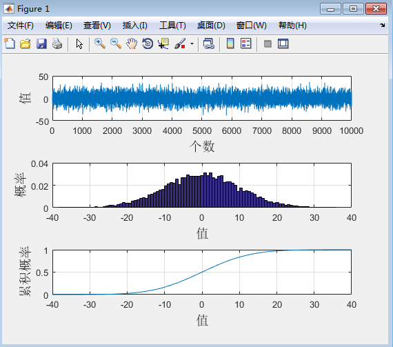
一、概率分布于累积概率分布

%概率分布函数和累积概率分布函数
clear
x = 10*randn([10000,1]);
xi = linspace(-40,40,201);

subplot(311)
plot(x)%原始数据
grid on
xlabel('个数','FontSize',14);%设置X坐标标签
ylabel('值','FontSize',14);%设置Y坐标标签

subplot(312)
[y,X]=hist(x,100);  %分为100个区间,统计每个区间个数)
y=y/length(x);   %计算概率密度 ，频数除以数据种数，除以组距
bar(X,y,1);  %用bar画图，最后的1是画bar图每条bar的宽度，默认是0.8所以不连续，改为1就可以了
grid on
xlim([-40 40]) %限定范围axis([xmin xmax ymin ymax])或者 ylim([ymin ymax])
xlabel('值','FontSize',14);%设置X坐标标签
ylabel('概率','FontSize',14);%设置Y坐标标签

%累计概率图
subplot(313)
F = ksdensity(x,xi,'function','cdf');
plot(xi,F);%累积概率函数图
grid on
xlabel('值','FontSize',14);%设置X坐标标签
ylabel('累积概率','FontSize',14);%设置Y坐标标签

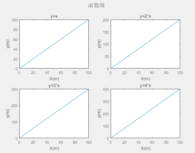
二、格式

clear all
h=0:0.1:100;
y1=h;
y2=2*h;
y3=3*h;
y4=4*h;

figure
subplot(221);
plot(h,y1)
title('y=x')
xlabel('X(m)')
ylabel('y(m)')

subplot(222);
plot(h,y2)
title('y=2*x')
xlabel('X(m)')
ylabel('y(m)')

subplot(223);
plot(h,y3)
title('y=3*x')
xlabel('X(m)')
ylabel('y(m)')

subplot(224);
plot(h,y4)
title('y=4*x')
xlabel('X(m)')
ylabel('y(m)')

suptitle('函数图')

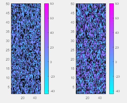
三、

两个colorbar 范围一致

clear all
k1=normrnd(10,10,50,50);
k2=normrnd(20,20,50,50);
subplot(1,2,2)
contourf(k2);
colormap(cool);
colorbar

k=caxis;
subplot(1,2,1);
contourf(k1)
caxis(k)
colorbar

四、

clear all

subplot(221)
x = [5 10];
y = [3 6];
C = [0 2 4 6; 8 10 12 14; 16 18 20 22];
imagesc(x,y,C)

subplot(222)
h2=subplot(222)
get(h2, 'Position')%得到位置
set(h2,'Position',[0.5303  0.5838 0.3347 0.3412])%调整位置
x = [5 10];
y = [3 6];
C = [0 2 4 6; 8 10 12 14; 16 18 20 22];
imagesc(x,y,C)

subplot(223)
x = [5 10];
y = [3 6];
C = [0 2 4 6; 8 10 12 14; 16 18 20 22];
imagesc(x,y,C)

h4=subplot(224)
get(h4, 'Position')%得到位置
set(h4,'Position',[0.5303  0.1100  0.3347 0.3412])
x = [5 10];
y = [3 6];
C = [0 2 4 6; 8 10 12 14; 16 18 20 22];
imagesc(x,y,C)

hBar = colorbar;
get(hBar, 'Position') %这样可以得到colorbar的左下角x,y坐标，以及宽和高。
set(hBar, 'Position', [0.9    0.23   0.0324    0.5405])
caxis([5,15])%颜色条范围限制
hBar.Label.String ='路径损失（dB）';%颜色柱表示含义
set(hBar.Label,'fontsize',10);%字段大小

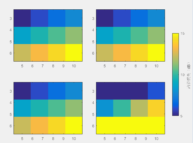
多个图合用一个颜色条，并且设置颜色条的位置，添加字体。

五、点图

clear all
x=[1:29];
y=ones(29);
figure
for i=1:15
    plot(x,y*i,'.', 'MarkerSize',20,'Color','k');
    hold on;
end
% axis([0 30 0 20]) %0坐标对不齐
%     grid on
axis equal
ylim([0 16])
xlim([0 30])

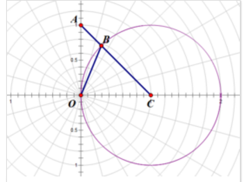
六、圆

极坐标系

极坐标系（polar coordinates）是指在平面内由极点、极轴和极径组成的坐标系。在平面上取定一点O，称为极点。从O出发引一条射线Ox，称为极轴。

再取定一个单位长度，通常规定角度取逆时针方向为正。这样，平面上任一点P的位置就可以用线段OP的长度ρ以及从Ox到OP的角度θ来确定，

有序数对（ρ，θ）就称为P点的极坐标，记为P（ρ，θ）；ρ称为P点的极径，θ称为P点的极角。

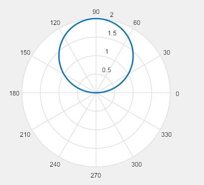
1、

figure
r=2; 
theta=0:pi/180:2*pi;%360度
x=r*cos(theta); 
y=r*sin(theta);
rho=r*sin(theta);
plot(x,y,'.','color','b')
%hold on; 
axis equal
%fill(x,y,'c')
figure
h=polar(theta,rho);
set(h,'LineWidth',2)

2、

clear all
figure
x=[1:29];
y=ones(29);
for i=1:15
    plot(x,y*i,'.', 'MarkerSize',20,'Color','k');
    hold on;
end
r=7; 
theta=0:pi/180:2*pi;%360度，360个点。
x=15+r*cos(theta); %（15,7.5）圆心
y=7.5+r*sin(theta);
rho=r*sin(theta);
plot(x,y,'.','color','b')

axis equal
ylim([0 16])
xlim([0 30]) %范围限制

转载于:https://www.cnblogs.com/ruo-li-suo-yi/p/9074094.html