机器学习多元线性回归_过度简化的机器学习（1）：多元回归

机器学习多元线性回归

The term machine learning may sound provocative. Machines do not learn like humans do. However, when given identifiable tasks to complete, machines excel.

机器学习一词听起来可能很挑衅。 机器不像人类那样学习。 但是，当完成可确定的任务后，机器就会表现出色。

Algorithms answer questions. Once trained they take in relevant information and give an educated guess to their question.

算法回答问题。 一旦接受培训，他们就会获取相关信息，并对问题进行有根据的猜测。

Let’s pretend you work for an advertising company that wants to identify a target audience for luxury items. The company won’t bother advertising to most consumers. So the company decides it wants to estimate salaries in Topeka, Kansas to find suitable targets for their marketing campaign. The firm finds a dataset online about local residents. This data is comprised of hours worked monthly, age, and monthly salary. The firm hopes to use this dataset to predict the salary of consumers not inside the dataset.

假设您在一家广告公司工作，该公司希望确定奢侈品的目标受众。 该公司不会打扰大多数消费者的广告。 因此，公司决定要估算堪萨斯州托皮卡的薪水，以便为其营销活动找到合适的目标。 该公司在线查找有关本地居民的数据集。 此数据包括每月工作时间，年龄和月薪。 该公司希望使用该数据集来预测不在该数据集中的消费者的工资。

Monthly Salary in Topeka, Kansas

堪萨斯州托皮卡的月薪

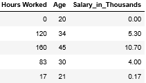
These first five examples contain monthly examples of descriptive information and salaries.

前五个示例包含描述性信息和薪水的每月示例。

It seems like there is a pattern to this data. Intuitively, if someone works more hours they are paid more. It also makes sense that older workers earn more because of their experience.

似乎此数据有模式。 凭直觉，如果某人工作时间更长，他们的工资就会更高。 同样有意义的是，老年工人由于他们的经验而获得更多的收入。

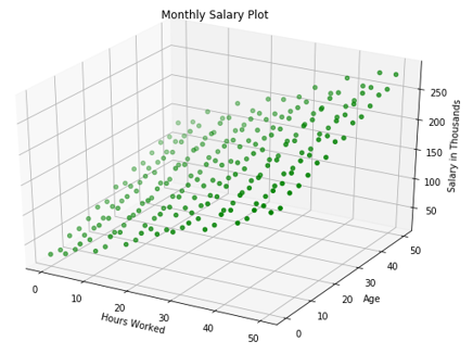
Let’s take a closer look at the entire dataset. A pattern emerges: both Age and Hours Worked increase salary.

让我们仔细看看整个数据集。 出现了一种模式：“年龄”和“工作时间”均增加薪水。

For each hour worked, salary on average increases by a certain amount. For every year of age salary on average increases by some other amount. The formula for this relationship looks like:

每工作一小时，工资平均增加一定数量。 对于每个年龄段，薪水平均增加一些其他金额。 这种关系的公式如下：

A + (Hours Worked * B) + (Age * C) = Salary

A +(工作时间* B)+(年龄* C)=工资

Where A, B, and C are unknown variables.

其中A，B和C是未知变量。

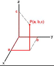
For every A, B, and C there exists a unique plane.

对于每个A，B和C，都有一个唯一的平面。

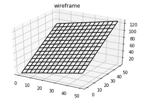
Let’s take the list of <A,B,C> and call it θ. Afterwards, let’s pick a random number for each. This creates a plane.

让我们以<A，B，C>的列表命名为θ。 之后，让我们为每个选择一个随机数。 这将创建一个平面。

This plane is like the bolded formula. It takes in two numbers and returns Z. Depending on the three numbers of Theta the plane takes a different shape.

这架飞机就像加粗的公式。 它采用两个数字并返回Z。根据Theta的三个数字，平面采用不同的形状。

Let’s use this randomly generated plane as an equation for the salary data. For every row in the dataset we create a single prediction.

让我们使用这个随机生成的平面作为薪水数据的方程式。 对于数据集中的每一行，我们创建一个预测。

Now we will establish a benchmark for the performance of the prediction. Lets take the difference between the prediction and actual salary columns, square every number, and sum them up:

现在，我们将为预测的性能建立基准。 让我们估算一下预测和实际工资列之间的差，对每个数字求平方，然后求和：

Cost(Salary_in_Thousands, Predicted Salary) = Sum((Salary_in_Thousands-Predicted Salary)²)

成本(千薪标准工资)=总和((千薪标准)²)

This benchmark for performance is called a cost function or loss function. The larger the sum, the larger the distance between the predictions and actual salaries.

此性能基准称为成本函数或损失函数。 总和越大，预测和实际薪水之间的距离越大。

Depending on the location of θ the model will be more or less accurate. In order to minimize the cost function we will need to adjust the values of θ.

根据θ的位置，模型将或多或少准确。 为了最小化成本函数，我们将需要调整θ的值。

.

。

The question remains: which direction do we move θ?

问题仍然存在：我们向哪个方向移动θ？

Gradient in Blue

蓝色渐变

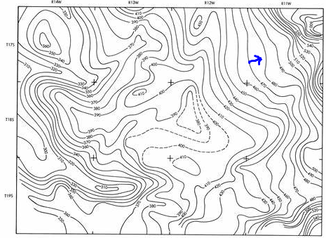
Contour maps show elevation using contour lines. Along these lines elevation is equal. Perpendicular to this is the line of steepest slope, called the gradient. Moving in this direction increases the Z value the fastest. By moving in the opposite direction the Z value decreases fastest.

等高线图使用等高线显示高程。 沿着这些线，海拔是相等的。 垂直于此的是最陡的斜率线，称为梯度 。 沿该方向移动将Z值最快地增加。 通过沿相反方向移动，Z值下降最快。

We will use the same idea to decrease error in our salary model. First, we calculate error as a function of θ.

我们将使用相同的想法来减少薪资模型中的错误。 首先，我们将误差计算为θ的函数。

Then we update θ using the following formula:

然后，使用以下公式更新θ：

θ = θ-∇Cost() … where ∇Cost() is the gradient

θ=θ-∇Cost()…其中∇Cost()是梯度

By subtracting the gradient we decrease the overall cost function and find a better θ. Because we are subtracting the gradient this method is called Gradient Descent.

通过减去梯度，我们降低了总成本函数并找到了一个更好的θ。 因为我们要减去梯度，所以此方法称为“ 梯度下降” 。

With our new θ we calculate the new predictions. We then calculate the new cost and new gradient. This leads to the following loop.

利用我们的新θ，我们可以计算出新的预测。 然后，我们计算新的成本和新的梯度。 这导致以下循环。

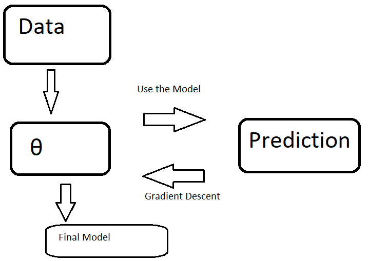
Once the cost is low enough we keep θ as our final model. For example, if the cost does not decrease for three straight loops, we can stop the process.

一旦成本足够低，我们将θ作为最终模型。 例如，如果成本没有连续三​​个循环下降，我们可以停止该过程。

We will use the final model to predict salaries of consumers in Topeka, Kansas using ages and workload of consumers. If our model predicts a high enough salary we will mark them as the target audience for our luxury brand adds.

我们将使用最终模型，根据消费者的年龄和工作量来预测堪萨斯州托皮卡的消费者工资。 如果我们的模型预测工资足够高，我们会将其标记为我们奢侈品牌的目标受众。

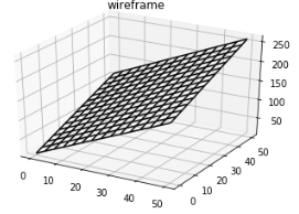
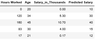
Here is our final model

这是我们的最终模型

Considering the original data, it is a strong approximation of the underlying pattern.

考虑到原始数据，它是基础模式的强近似值。

This is a graph representing our model.

这是代表我们模型的图形。

θ[0] is the first variable of θ.

θ[0]是θ的第一个变量。

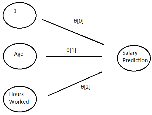
The left represents the inputs to the model: age and hours worked.

左侧代表模型的输入：年龄和工作时间。

The data moves from the left to the right through three channels. The wider the channel, indicated by θ[i], the larger the output to the right. The top line represents 1*θ[0]

数据通过三个通道从左到右移动。 通道越宽，用θ[i]表示，右侧的输出越大。 第一行代表1 *θ[0]

The right hand side is the output of the model. It is the sum of each input multiplied by its θ.

右侧是模型的输出。 它是每个输入的总和乘以其θ。

The math is written as <1, age, hours worked>*θ = Salary Prediction

数学写为<1，年龄，工作小时数> *θ=工资预测

Check out part 2 here:

在这里查看第2部分：

翻译自: https://medium.com/data-for-associates/oversimplified-ml-1-multiple-regression-eaf49fee7aa1

机器学习多元线性回归