正态分布随机概率算法_减少维t分布随机邻居嵌入的概率算法-优快云博客

本文深入探讨了t-SNE算法的工作原理及其在数据可视化中的应用。对比PCA，t-SNE能更好地处理非线性数据，并保留数据的局部结构。文章还介绍了如何使用Python对MNIST数据集执行t-SNE。

摘要生成于 C知道，由 DeepSeek-R1 满血版支持，前往体验 >

正态分布随机概率算法

数据可视化(Data Visualization)

Data Visualization plays a crucial role in real-time Machine Learning applications. Visualizing data makes a much easier and convenient way to know, interpret, and classify data in many cases. And there are some techniques which can help to visualize data and reduce dimensions of the dataset.

数据可视化在实时机器学习应用程序中扮演着至关重要的角色。在许多情况下，可视化数据将为了解，解释和分类数据提供一种更加轻松便捷的方法。并且有一些技术可以帮助可视化数据并减少数据集的维度。

In my previous article, I gave an overview of Principal Component Analysis (PCA) and explained how to implement it. PCA is a basic technique to reduce dimensions and plot data. There are some limitations of using PCA from which the major is, it does not group similar classes together rather it is just a method of transforming point to linear representation which makes it easier for humans to understand data. While t-SNE is designed to overcome this challenge such that it can group similar objects together even in a context of lack of linearity.

在上一篇文章中，我概述了主成分分析(PCA)并解释了如何实现它。 PCA是减少尺寸和绘制数据的基本技术。使用PCA的专业存在一些局限性，它不会将相似的类组合在一起，而只是将点转换为线性表示的一种方法，使人类更容易理解数据。尽管t-SNE旨在克服这一挑战，即使在缺乏线性的情况下，它也可以将相似的对象组合在一起。

This article is categorized into the following sections:

本文分为以下几节：

What is t-SNE?
什么是t-SNE？
Need/Advantages of t-SNE
t-SNE的需求/优势
Drawbacks of t-SNE
t-SNE的缺点
Applications of t-SNE — when to use and when not to use?
t-SNE的应用-什么时候使用和什么时候不使用？
Implementation of t-SNE to MNIST dataset using Python
使用Python对MNIST数据集执行t-SNE
Conclusion
结论

什么是t-SNE？(What is t-SNE?)

It is a technique that tries to maintain the local structure of the data-points which reduces dimensions.

它是一种尝试维护数据点的局部结构的技术，从而减小了尺寸。

Let’s understand the concept from the name (t — Distributed Stochastic Neighbor Embedding): Imagine, all data-points are plotted in d -dimension(high) space and a data-point is surrounded by the other data-points of the same class and another data-point is surrounded by the similar data-points and of same class and likewise for all classes. So now, if we take any data-point (x) then the surrounding data-points (y, z, etc.) are called the neighborhood of that data-point, neighborhood of any data-point (x) is calculated such that it is geometrically close with that neighborhood data-point (y or z), i.e. by calculating the distance between both data-points. So basically, the neighborhood of x contains points that are closer to x. The technique only tries to preserve the distance of the neighborhood.

让我们从名称(t －分布式随机邻居嵌入)中了解概念：想象一下，所有数据点都在d维(高)空间中绘制，并且一个数据点被相同类别的其他数据点包围，并且另一个数据点被相似的数据点所包围，并且属于同一类，并且所有类同样如此。因此，现在，如果我们取任何数据点(x)，则将周围的数据点(y，z等)称为该数据点的邻域，计算出任何数据点(x)的邻域，使得它在几何上与该邻域数据点(y或z)接近，即通过计算两个数据点之间的距离。因此，基本上，x的邻域包含更接近x的点。该技术仅尝试保留邻域的距离。

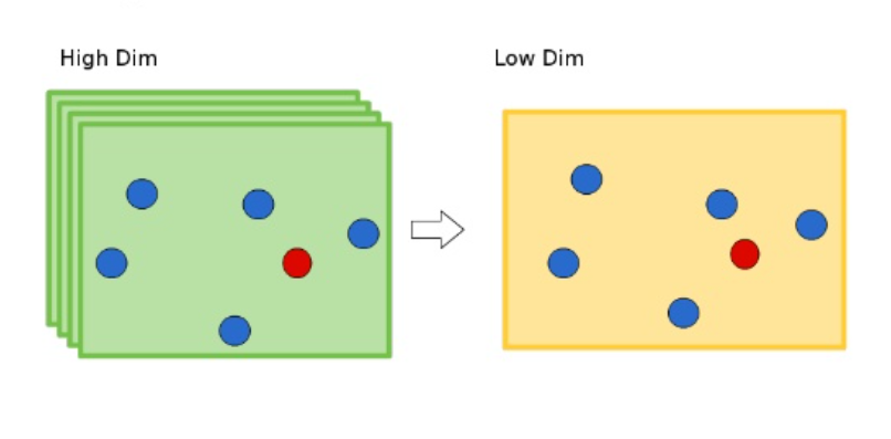
What is embedding? The data-points plotted in d-dimension are embedded in 2D such that the neighborhood of all data-points are tried to maintain as they were in d-dimension. Basically, for every point in high dimension space, there’s a corresponding point in low dimension space with the neighborhood concept of t-SNE.

嵌入什么？ 以d维绘制的数据点被嵌入2D中，以便尝试保持所有数据点的邻域与d维相同。基本上，对于高维空间中的每个点，在低维空间中都有一个对应的点，具有t-SNE的邻域概念。

t-SNE creates a probability distribution using the Gaussian distribution that defines the relationships between the points in high-dimensional space.

t-SNE使用高斯分布创建概率分布，该概率分布定义了高维空间中各点之间的关系。

It is stochastic since in every run it’s output changes, that is it is not deterministic.

这是随机的，因为在每次运行中它的输出都会变化，也就是说，它不是确定性的。

为什么我们需要t-SNE？ (Why do we need t-SNE?)

Handles non-linearity: When it comes to dimensionality reduction, PCA is widely used as it is easy to use and understand intuitively. It tries to preserve linearity to the dataset by maintaining the spread(variance) of the data-points. PCA is a linear algorithm. It creates Principal Components which are the linear combinations of the existing features. So, it is not able to interpret complex polynomial relationships between features. So, if the relationship between the variables is nonlinear, it performs poorly. On the other hand, t-SNE works well on non-linear data. The main objective of t-SNE is to maintain non-linearity of the data-points which can be helpful in overcoming challenges of PCA for some applications.
处理非线性：在降维方面，由于易于使用和直观理解，PCA被广泛使用。它试图通过保持数据点的散布(方差)来保持数据集的线性。 PCA是一种线性算法。它创建主要组件，这些组件是现有特征的线性组合。因此，它无法解释要素之间的复杂多项式关系。因此，如果变量之间的关系是非线性的，则其性能会很差。另一方面，t-SNE在非线性数据上效果很好。 t-SNE的主要目标是保持数据点的非线性，这有助于克服某些应用中PCA的挑战。
Preserves local and global structure: t-SNE is capable of preserving the local and global structure of the data. This means, roughly, that points which are close to one another in the high-dimensional dataset, will tend to be close to one another in the low dimension. On the other hand, PCA finds new dimensions that explain most of the variance in the data. So, it cares relatively little about local neighbors, unlike t-SNE.
保留本地和全局结构： t-SNE能够保留数据的本地和全局结构。粗略地讲，这意味着在高维数据集中彼此接近的点在低维方向上趋于彼此接近。另一方面，PCA可以找到新的维度来解释数据中的大部分差异。因此，与t-SNE不同，它对本地邻居的关心相对较少。

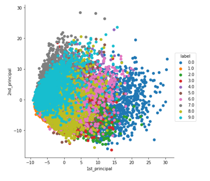
The above graph shows the final output on the MNIST dataset after implementing PCA.

上图显示了实施PCA之后，MNIST数据集上的最终输出。

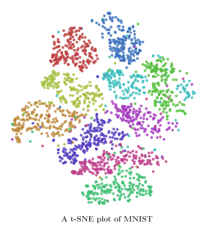
The above graph depicts the final output on the MNIST dataset after implementing t-SNE.

上图描述了实施t-SNE之后在MNIST数据集上的最终输出。

t-SNE的缺点 (Drawbacks of t-SNE)

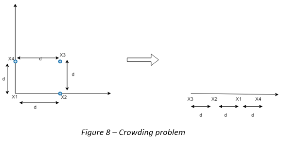
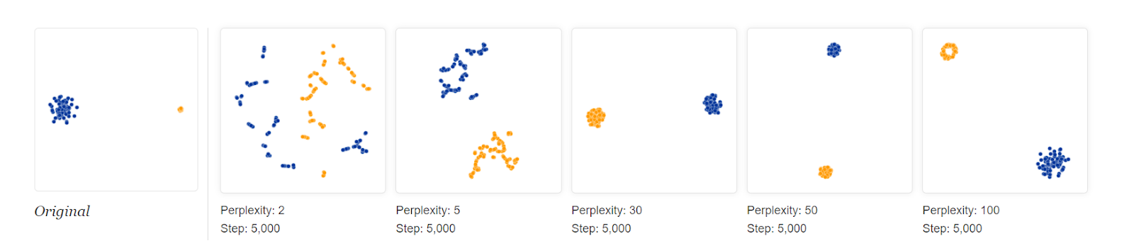
Crowding Problem: Let’s suppose a square of points a, b, c, and d with length x is represented in 2D and now applying t-SNE, one wants to reduce dimensions to 1D, first a is represented on a line, now point b is represented on the left of point a at x distance and point c is plotted on the right of a point at x distance. Here, the neighborhood of a are preserved but one can’t preserve the distance between point b and point c.
拥挤问题：让我们假设以2D表示长度为x的点a，b，c和d的正方形，然后应用t-SNE，一个人希望将尺寸减小为1D，首先将a表示在一条线上，现在点b表示在x距离的点a的左侧，而在c距离的点的右侧绘制c。在这里，保留了a的邻域，但不能保留b点和c点之间的距离。

Computationally Complex: t-SNE involves a lot of calculations and computations because it computes pairwise conditional probabilities for each data point and tries to minimize the sum of the difference of the probabilities in higher and lower dimensions.
计算复杂： t-SNE涉及大量计算和计算，因为它为每个数据点计算成对条件概率，并尝试最大程度地减小上下维度的概率之和。
Selection of Hyperparameters: Perplexity and Steps (will come later in the article)
选择超参数：困惑和步骤(将在本文后面)
Cluster size: t-SNE does not consider the cluster size of any classes.
群集大小： t-SNE不考虑任何类别的群集大小。

t-SNE的应用 (Applications of t-SNE)

t-SNE could be used on high-dimensional data and then the output of those dimensions then become inputs to some other classification model. Also, t-SNE could be used to investigate, learn, or evaluate segmentation. Oftentimes one selects the number of segments prior to modeling or iterates after results. t-SNE can oftentimes show clear separation in the data. This can be used prior to using your segmentation model to select a cluster number or after to evaluate if your segments actually hold up. t-SNE however is not a clustering approach since it does not preserve the inputs like PCA and the values may often change between runs so it’s purely for exploration. It is used to interpret deep neural network outputs in tools such as the TensorFlow Embedding Projector and TensorBoard, a powerful feature of tSNE is that it reveals clusters of high-dimensional data points at different scales while requiring only minimal tuning of its parameters. It is widely used for Deep Learning applications.

t-SNE可以用于高维数据，然后这些维的输出将成为其他分类模型的输入。同样，t-SNE可用于研究，学习或评估细分。通常会在建模之前选择段的数量，或在结果之后进行迭代。 t-SNE通常可以显示清楚的数据分离。可在使用细分模型选择集群编号之前或在评估细分是否真正成立之后使用此方法。但是，t-SNE并不是一种聚类方法，因为它不保留PCA之类的输入，并且值通常在运行之间可能会发生变化，因此它仅用于探索。它用于解释TensorFlow嵌入式投影仪和TensorBoard等工具中的深层神经网络输出， tSNE的强大功能在于，它可以显示不同比例的高维数据点簇，而只需要对其参数进行最小的调整。它被广泛用于深度学习应用。

使用Python实现t-SNE到MNIST数据集 (Implementation of t-SNE to MNIST dataset using Python)

To download the MNIST dataset, from data. First, we will load as well as understand columns and data-points. Also, separate the label column from the CSV file and store it in another dataframe.

要下载MNIST数据集，从数据。首先，我们将加载并理解列和数据点。另外，将标签列与CSV文件分开，并将其存储在另一个数据框中。

# MNIST dataset downloaded from Kaggle : 
# https://www.kaggle.com/c/digit-recognizer/data




#importing libraries
import numpy as np
import pandas as pd
import matplotlib.pyplot as plt


#loading/reading csv file 
data = pd.read_csv('/content/train.csv')


print(data.head(5)) # print first five rows of data.


#seperating x-matrix(features) and y-matrix(labels) by storing in different dataframes
# save the labels into a label dataframe.
label = data['label']
print(label.head(5))
print(type(label))


# Drop the label feature and store the pixel data(features) in feature.
feature = data.drop("label",axis=1)
print(feature.head(5))
print(type(feature))

Now, as a part of Data Preprocessing, we’ll standardize data as follows:

现在，作为数据预处理的一部分，我们将数据标准化如下：

# Data-preprocessing: Standardizing the data


from sklearn.preprocessing import StandardScaler


standardized_data = StandardScaler().fit_transform(feature)
print(standardized_data.shape)

The next step is to implement t-SNE using Sk-learn.

下一步是使用Sk-learn实现t-SNE。

Here, we’ll use the first 1000 standardized data-points for t-SNE. And prepare a model of t-SNE from the sklearn module using some default parameters. It is advisable to apply different perplexity, learning-rate to classify labels in a better way. Moreover, we’ll fit and transform the t-SNE model and plot that using seaborn as follows:

在这里，我们将使用t-SNE的前1000个标准化数据点。并使用一些默认参数从sklearn模块准备t-SNE模型。建议应用不同的困惑度和学习率，以更好的方式对标签进行分类。此外，我们将拟合并转换t-SNE模型，并使用seaborn进行如下绘制：

# TSNE # https://scikit-learn.org/stable/modules/generated/sklearn.manifold.TSNE.html
import seaborn as sns
from sklearn.manifold import TSNE


# Picking the top 1000 points as TSNE takes a lot of time for 15K points
data_1000 = standardized_data[0:1000, :]
labels_1000 = labels[0:1000]


model = TSNE(n_components = 2, random_state = 0)
# configuring the parameteres
# the number of components = 2 -> dimensions of the embedded space.
# default perplexity = 30 -> erplexity is related to the number of nearest neighbors that is used in other manifold learning algorithms.
# default learning rate = 200 -> The learning rate for t-SNE is usually in the range [10.0, 1000.0]. If the learning rate is too high, the data may look like a ‘ball’ with any point approximately equidistant from its nearest neighbours. If the learning rate is too low, most points may look compressed in a dense cloud with few outliers. If the cost function gets stuck in a bad local minimum increasing the learning rate may help.
# default Maximum number of iterations for the optimization = 1000


tsne_data = model.fit_transform(data_1000)




# creating a new data frame which help us in ploting the result data
tsne_data = np.vstack((tsne_data.T, labels_1000)).T #https://numpy.org/doc/stable/reference/generated/numpy.vstack.html
tsne_df = pd.DataFrame(data = tsne_data, columns = ("Dim_1", "Dim_2", "label")) #https://seaborn.pydata.org/generated/seaborn.FacetGrid.html


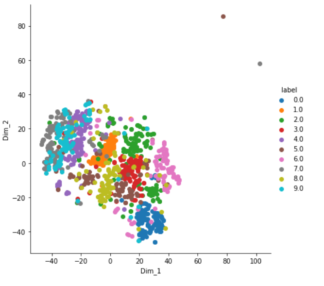
# Ploting the result of tsne
sns.FacetGrid(tsne_df, hue = "label", size=6).map(plt.scatter, 'Dim_1', 'Dim_2').add_legend()
plt.show()

Output:

输出：

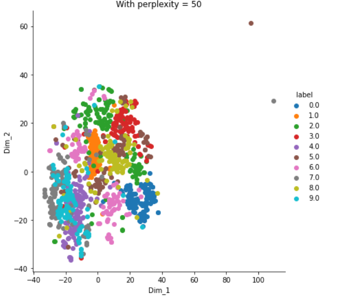
Trying with perplexity = 50;

困惑尝试= 50;

model = TSNE(n_components = 2, random_state = 0, perplexity = 50)
tsne_data = model.fit_transform(data_1000) 


# creating a new data fram which help us in ploting the result data
tsne_data = np.vstack((tsne_data.T, labels_1000)).T
tsne_df = pd.DataFrame(data=tsne_data, columns=("Dim_1", "Dim_2", "label"))


# Ploting the result of tsne
sns.FacetGrid(tsne_df, hue="label", size=6).map(plt.scatter, 'Dim_1', 'Dim_2').add_legend()
plt.title('With perplexity = 50')
plt.show()

Output: This looks very similar to the above plot with perplexity = 30.

输出：这看起来与上面的图非常相似，困惑度= 30。

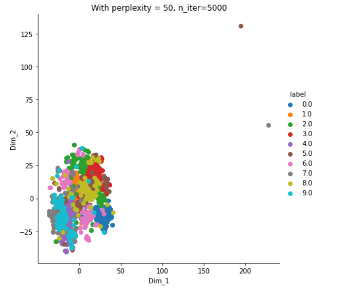
Trying t-SNE with 5000 iterations instead of 1000;

用5000次迭代而不是1000次尝试t-SNE；

model = TSNE(n_components=2, random_state=0, perplexity=50,  n_iter=5000)
tsne_data = model.fit_transform(data_1000) 


# creating a new data fram which help us in ploting the result data
tsne_data = np.vstack((tsne_data.T, labels_1000)).T
tsne_df = pd.DataFrame(data=tsne_data, columns=("Dim_1", "Dim_2", "label"))


# Ploting the result of tsne
sns.FacetGrid(tsne_df, hue="label", size=6).map(plt.scatter, 'Dim_1', 'Dim_2').add_legend()
plt.title('With perplexity = 50, n_iter=5000')
plt.show()

Output:

输出：

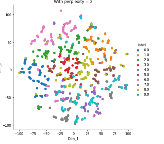
Now, with perplexity = 2

现在，困惑度= 2

model = TSNE(n_components = 2, random_state = 0, perplexity = 2)
tsne_data = model.fit_transform(data_1000) 


# creating a new data fram which help us in ploting the result data
tsne_data = np.vstack((tsne_data.T, labels_1000)).T
tsne_df = pd.DataFrame(data=tsne_data, columns=("Dim_1", "Dim_2", "label"))


# Ploting the result of tsne
sns.FacetGrid(tsne_df, hue = "label", size = 6).map(plt.scatter, 'Dim_1', 'Dim_2').add_legend()
plt.title('With perplexity = 2')
plt.show()

Output: All of the information is lost, all data-points are randomly spread as follows;

输出：所有信息丢失，所有数据点按以下方式随机分布；

结论 (Conclusion)

We need to try different values of perplexity and the number of iterations in order to find the best solution. Try to implement t-SNE with all data-points(it will take some time to execute).

我们需要尝试不同的困惑度值和迭代次数才能找到最佳解决方案。尝试用所有数据点实现t-SNE(这将需要一些时间来执行)。

You can find the source code from Github

您可以从Github找到源代码

If you have confusion regarding any function/class of the library, then I request you to check the documentation for that.

如果您对库的任何功能/类有疑问，请联系我们查阅文档。

If there’s any correction & scope of improvement or if you have any queries, let me know at Mail / LinkedIn.

如果有任何更正和改进的范围，或者您有任何疑问，请通过Mail / LinkedIn告诉我。

For a detailed understanding of drawbacks, check out: https://distill.pub/2016/misread-tsne/

要详细了解缺点，请查看： https : //distill.pub/2016/misread-tsne/

For the application of t-SNE, check out: https://ai.googleblog.com/2018/06/realtime-tsne-visualizations-with.html

对于t-SNE的应用程序，请查看： https : //ai.googleblog.com/2018/06/realtime-tsne-visualizations-with.html