


简化日志输出
What can we predict with a neural network?
我们可以用神经网络预测什么?
Let’s say you want to be involved in AI but don’t know how to code. It is important to remember when a neural network is applicable and when it isn’t. Neural networks use data in order to create an output. We are going to skip the ‘how it works’ part. Instead we will only focus on what we are capable of creating.
假设您想参与AI,但不知道如何编码。 重要的是要记住何时可以使用神经网络,什么时候不可以。 神经网络使用数据来创建输出。 我们将跳过“工作原理”部分。 相反,我们将只专注于我们能够创造的东西。
You might be familiar with the black box approach to machine learning. This approach simplifies an algorithm into three pieces: the inputs, the model, and the outputs. Since we are skipping how to create a model, we will just replace it with a black box.
您可能熟悉机器学习的黑匣子方法。 这种方法将算法简化为三部分:输入,模型和输出。 由于我们跳过了创建模型的过程,因此我们将其替换为黑框。
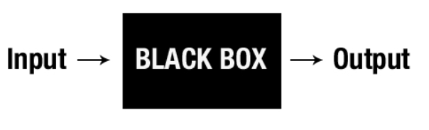
Once we know how to train a model/network, it doesn’t really matter why it works. The more important aspect is understanding what questions we are capable of answering.
一旦我们知道了如何训练模型/网络,它为什么起作用就没有关系了。 更重要的方面是了解我们能够回答哪些问题。
Regression
回归
The first type of output is a decimal number. A model which outputs a decimal is called a regression model. When the variable we want to predict could be anywhere on the number line we will use a regression model. This type of output is called a continuous variable.
第一类输出是十进制数。 输出小数的模型称为回归 模型。 当我们要预测的变量可能在数字线上的任意位置时,我们将使用回归模型。 这种类型的输出称为连续变量。
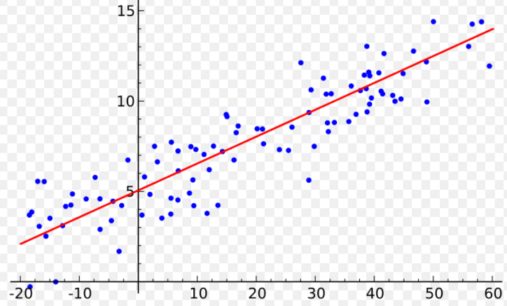
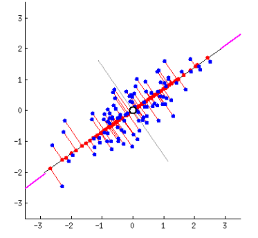
An example of a regression model is a line through (x,y) data points. Given an input (x) the model returns an output (y). This output could be anywhere from -infinity to +infinity.
回归模型的一个示例是穿过(x,y)数据点的直线。 给定输入(x),模型返回输出(y)。 此输出的范围可以是-infinity到+ infinity。
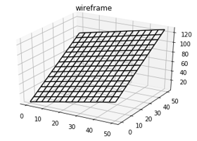
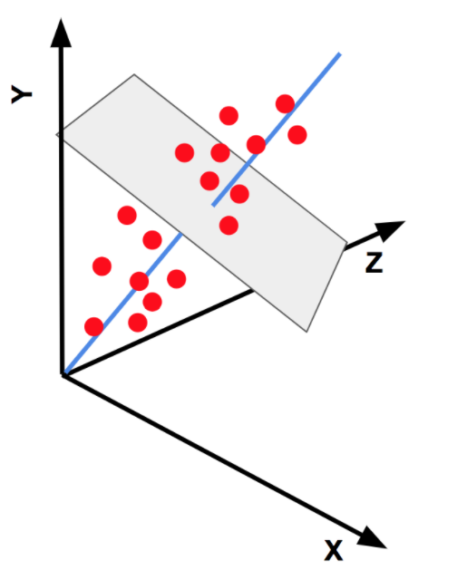
If we have multiple inputs a regression model looks like a plane:
如果我们有多个输入,则回归模型看起来像一个平面:
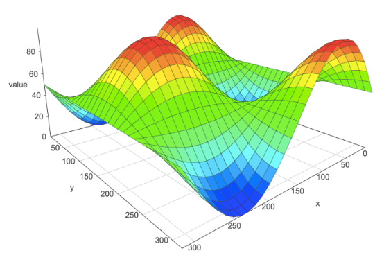
An advanced regression model will look something like the image to the left. A neural network is capable of creating any surface in order to match data.
高级回归模型的外观类似于左侧的图像。 神经网络能够创建任何表面以匹配数据。
We can create a prediction by plugging in the inputs (x,y) and returning the corresponding value.
我们可以通过插入输入(x,y)并返回相应的值来创建预测。
Classification
分类
The second type of output is a class. A class is a group that has certain characteristics. There is no limit to the number of members in a class. Neural networks are capable of classifying data points into distinct classes by outputting a whole number.
输出的第二种类型是类。 类是具有某些特征的组。 对班级成员的数量没有限制。 神经网络能够通过输出整数将数据点分类为不同的类。
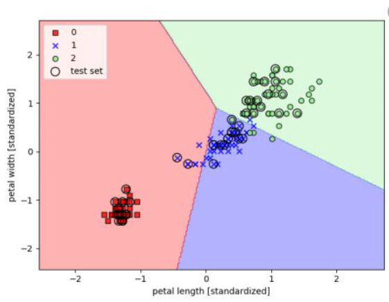
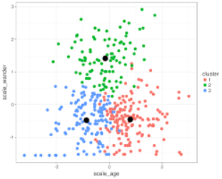
In this example we classify flowers according to petal length and petal width. The network outputs a zero when the data point is in the red section, a one in the blue section, and a two in the green section.
在此示例中,我们根据花瓣长度和花瓣宽度对花朵进行分类。 当数据点在红色部分时,网络输出零;在蓝色部分中,数据点输出一;在绿色部分,网络输出2。
Another example of classification is spam detection. Using the words of an email a computer can predict if an email is spam. Once spam is identified it is put aside in the trash folder.
分类的另一个示例是垃圾邮件检测。 使用电子邮件中的单词,计算机可以预测电子邮件是否为垃圾邮件。 一旦识别出垃圾邮件,就会将其放在垃圾箱文件夹中。
Another Data set
另一个数据集
The third type of output from a model is an altered data set. Sometimes data sets require processing before use in regression or classification. This is especially true of “wide” datasets with many columns. This type of machine learning will reduce the number of columns until the data set is more manageable.
模型输出的第三种类型是更改后的数据集。 有时,数据集需要进行处理才能用于回归或分类。 对于具有许多列的“宽”数据集尤其如此。 这种类型的机器学习将减少列数,直到数据集更易于管理为止。
One method to simplify data is called principal component analysis, or PCA.
一种简化数据的方法称为主成分分析或PCA。
This method assigns a line through data that best represents it. Points are then moved across the orthogonal (diagonal) line to the line of best fit.
此方法通过最能代表其的数据分配一条线。 然后,将点跨过正交(对角线)移动到最佳拟合线。
After moving this process each point can be represented with two new values. Instead of (x,y) defining a data point PCA will represent each point with the position on the line of best fit and the orthogonal distance. Since the line of best fit comes first, the first number will be more significant than the second.
移动此过程后,可以用两个新值表示每个点。 代替定义(x,y),数据点PCA将用最佳拟合线上的位置和正交距离表示每个点。 由于最佳拟合线排在第一位,因此第一个数字将比第二个数字更重要。
In 3D and higher dimensions we largely follow the same process.
在3D和更高尺寸中,我们很大程度上遵循相同的过程。
To start, we choose the line which has the lowest orthogonal squared error. This is the sum of the length of each orthogonal line squared.
首先,我们选择具有最小正交平方误差的线。 这是每条正交线长度平方的总和。
Next, each point’s first principal component is recorded. This is done by finding the intercept between the line of best fit and the orthogonal distance. The distance along the line of best fit is the first principal component. A point in the top right would have a large first component while a point closer to (0,0,0) has a smaller first principal component.
接下来,记录每个点的第一个主要成分。 这是通过找到最佳拟合线和正交距离之间的截距来完成的。 沿着最佳拟合线的距离是第一个主要成分。 右上方的点将具有较大的第一成分,而更接近(0,0,0)的点将具有较小的第一主成分。
After the first principal component is collected all points are moved to the perpendicular plane. Another line of best fit is calculated and the second principal component is derived. This process is repeated until only one dimension is left. That dimension becomes the final principal component.
收集第一个主成分后,所有点都移到垂直平面。 计算另一条最佳拟合线,并得出第二个主要成分。 重复此过程,直到只剩下一个尺寸。 该维度成为最终的主要组成部分。
The data set is now described with the most important variables first and the least important variables last. We can safely remove the least important variables without losing much of the original information.
现在描述数据集,首先是最重要的变量,最后是最不重要的变量。 我们可以安全地删除最不重要的变量,而不会丢失很多原始信息。
To explore how efficient our transformation is we need to compare the new and old data sets. To compare these data sets they must be in the same dimensions.
为了探索转换的效率,我们需要比较新的和旧的数据集。 为了比较这些数据集,它们必须具有相同的维度。
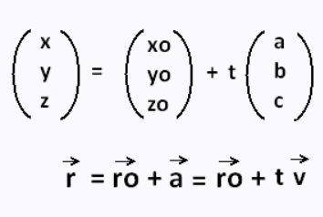
Using the equation for a line we are able to return to the old data’s dimensions for each point. Plug in the first component’s value in for t. The other variables come from the line used in PCA.
使用一条线的方程式,我们可以返回每个点的旧数据尺寸。 将第一个组件的值插入t中。 其他变量来自PCA中使用的行。
Repeat this process for the first k number of columns in the PCA data set. Now we have x (the original point) and x_approx (the new point in x dimensions).
对PCA数据集中的前k个列重复此过程。 现在我们有了x(原始点)和x_approx(x维度中的新点)。
To measure how much information is lost we will look at the variance before and after the transformation. If we have lost too much variance we should add another column from PCA. If we still have almost all the variance we can ‘simplify’ the data by removing the rightmost column of PCA. Repeat until an acceptable amount of variance and number of columns is reached
为了衡量丢失了多少信息,我们将查看转换前后的方差。 如果我们损失了太多的差异,则应从PCA中添加另一列。 如果我们仍然拥有几乎所有的方差,我们可以通过删除PCA的最右列来“简化”数据。 重复直到达到可接受的方差量和列数
Clusters
集群
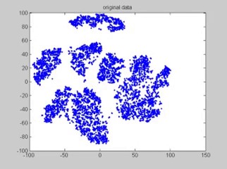
The fourth output of an algorithm is clustering. Clustering assigns every point a group. Each group has certain characteristics and, if done properly, any member of the same group has similar characteristics.
算法的第四项输出是聚类。 聚类为每个点分配一个组。 每个组都有某些特征,如果做得正确,同一组的任何成员都具有相似的特征。
One of the most popular methods for clustering data is k-means. This process creates a number of hot spots and assigns data to whichever spot is closest.
k-means是最流行的数据聚类方法之一。 此过程将创建多个热点,并将数据分配给最接近的那个热点。
This is a five step process. First, we randomly choose three points from our data set. These will be the starting locations for our hot spots.
这是一个五步过程。 首先,我们从数据集中随机选择三个点。 这些将是我们热点的起点。
Second, we ask every point in the data set which hot spot it is closest to. This will be the point’s cluster.
其次,我们要求数据集中的每个点最接近哪个热点。 这将是该点的群集。
Third, we ask each hot spot which direction it should move in to be closest to its assigned points. We will take a small step in this direction so that each hot spot is placed more efficiently.
第三,我们询问每个热点应朝哪个方向移动,使其最接近其指定点。 我们将朝这个方向迈出一小步,以便更有效地放置每个热点。
Fourth, we repeat steps two and three until we have a strong clustering system. As we repeat these steps the clustering becomes a better and better fit to our data. Once the distances between points and their hot spots stop decreasing we record each hot spot’s location and the sum of distances between points and their respective hot spots.
第四,我们重复步骤2和3,直到拥有一个强大的集群系统。 随着我们重复这些步骤,聚类变得越来越适合我们的数据。 一旦点与热点之间的距离停止减小,我们就会记录每个热点的位置以及点与各自热点之间的距离之和。
Fifth, we repeat steps one through four. Since the initial hot spots are randomly chosen we converge to different solutions. Once we have run this algorithm 20+ times we should choose the best one. The best clustering algorithm has the smallest sum of distances to each point’s respective hot spot.
第五,我们重复第一步到第四步。 由于初始热点是随机选择的,因此我们可以收敛到不同的解决方案。 一旦运行了20次以上,我们应该选择最佳算法。 最佳的聚类算法具有到每个点相应热点的最小距离总和。
Now you have learned what machine learning algorithms can create.
现在,您已经了解了可以创建什么机器学习算法。
翻译自: https://medium.com/data-for-associates/oversimplified-ml-3-outputs-d987ccc71737
简化日志输出


 被折叠的 条评论
为什么被折叠?
被折叠的 条评论
为什么被折叠?
 到【灌水乐园】发言


