攻防演练_了解lenet详细的演练

攻防演练

了解CNN(Understanding CNNs)

目录 (Table of Contents)

1. An Overview of LeNet

   LeNet概述

2. Convolutional Neural Network Basics

   卷积神经网络基础

3. A Walkthrough of LeNet-1’s Architecture

   LeNet-1体系结构的演练

4. A Walkthrough of LeNet-4’s Architecture

   LeNet-4体系结构的演练

5. A Walkthrough of LeNet-5’s Architecture

   LeNet-5体系结构的演练

6. Analysis of LeNet

   LeNet分析

7. Summary of LeNet

   LeNet的摘要

1. LeNet概述(1. An Overview of LeNet)

LeNet was a group of Convolutional Neural Networks (CNNs) developed by Yann Le-Cun and others in the late 1990s. The networks were broadly considered as the first set of true convolutional neural networks. They were capable of classifying small single-channel (black and white) images, with promising results. LeNet consisted of three distinct networks, and they were:

LeNet是由Yann Le-Cun和其他人在1990年代后期开发的一组卷积神经网络(CNN)。 该网络被广泛认为是第一批真正的卷积神经网络。 他们能够对小型单通道(黑白)图像进行分类，并取得了可喜的结果。 LeNet由三个不同的网络组成，分别是：

1. LeNet-1 (five layers): A simple CNN.
   LeNet-1(五层)：一个简单的CNN。
2. LeNet-4 (six layers): An improvement over LeNet-1.
   LeNet-4(六层)：对LeNet-1的改进。
3. LeNet-5 (seven layers): An improvement over LeNet-4 and the most popular.
   LeNet-5(七层)：是对LeNet-4的改进，并且是最流行的。

2.卷积神经网络基础 (2. Convolutional Neural Network Basics)

Convolutional Neural Networks were initially designed to mimic the biological processes of human vision. The networks utilised multiple layers that were ordered in different ways to form distinct network architectures. The three types of layers that traditional neural networks included were:

卷积神经网络最初旨在模拟人类视觉的生物过程。 网络利用以不同方式排序的多层来形成不同的网络体系结构。 传统神经网络包括的三种类型的层是：

1. Convolution Layers
   卷积层
2. Subsampling Layers
   二次采样层
3. Fully Connected Layers
   完全连接的层

卷积层(Convolution Layers)

Two-dimensional convolution layers used trainable kernels or filters to perform convolution operations, sometimes including an optional trainable bias for each kernel. These convolution operations involved moving the kernels over the input in steps called strides. Generally, the larger the stride was, the more spaces the kernels skipped between each convolution. This led to less overall convolutions and more miniature output size. For each placement of a given kernel, a multiplication operation was performed between the input section and the kernel, with the bias summed to the result. This produced a feature map containing the convolved result. The feature maps were typically passed through an activation function to provide input for the subsequent layer. The size of the feature map was calculated as [(input_size − kernel_size + 2 × padding) / stride] + 1.

二维卷积层使用可训练的内核或过滤器执行卷积运算，有时会为每个内核包括一个可选的可训练偏差。 这些卷积操作涉及以步幅为步长在输入上移动内核。 通常，跨度越大，内核在每个卷积之间跳过的空间就越大。 这导致更少的整体卷积和更大的输出尺寸。 对于给定内核的每个放置，在输入部分和内核之间执行乘法运算，并向结果求和。 这产生了包含卷积结果的特征图。 特征图通常通过激活函数传递，以为后续层提供输入。 特征图的大小计算为[(input_size − kernel_size + 2×padding)/ stride] + 1。

Figure 2: Convolution Operation Example (image by author)

图2：卷积运算示例(作者提供的图片)

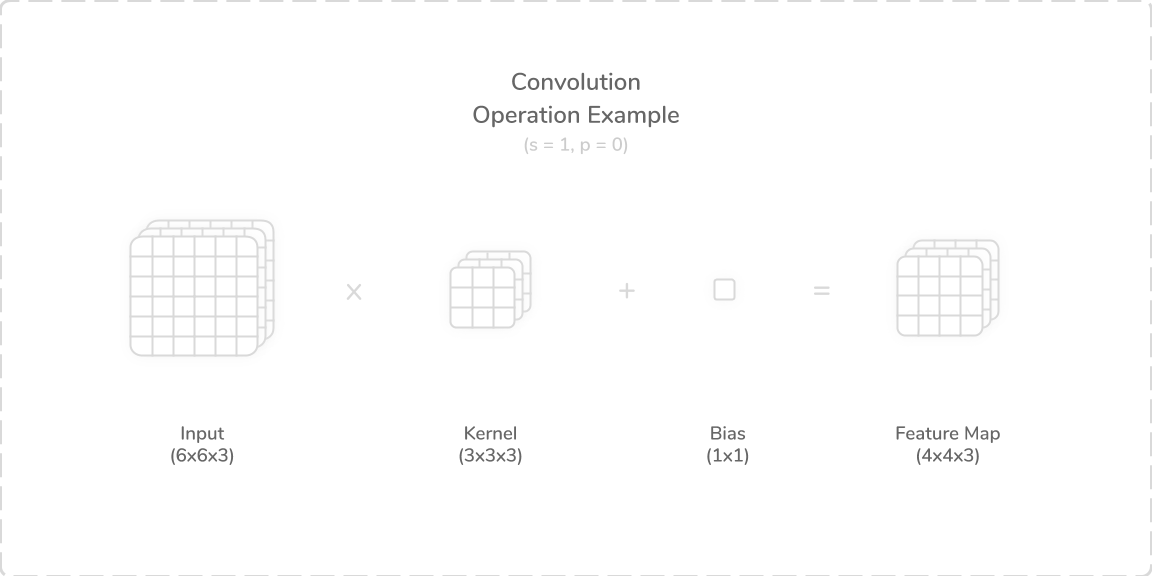
Figure 2 shows a convolution operation that involved a 3-channel (6×6) image, a 3-channel (3×3) kernel and a (1×1) bias. The operation was implemented with a stride of one and zero padding. This meant that the kernel moved over each (3×3) section of the image in an overlapping left-to-right motion, shifting one place between each operation. This resulted in a 3-channel (4×4) convolved feature map. Generally, the number of kernel channels was always identical to the number of input channels.

图2显示了涉及3通道(6×6)图像，3通道(3×3)内核和(1×1)偏差的卷积运算。 该操作的执行跨度为一填充和零填充。 这意味着内核以从左到右的重叠运动在图像的每个(3×3)区域上移动，在每个操作之间移动了一个位置。 这产生了3通道(4×4)卷积特征图。 通常，内核通道的数量始终与输入通道的数量相同。

二次采样层 (Subsampling Layers)

Two-dimensional subsampling layers used non-trainable kernels or windows to down-sample input features. This typically reduced the size of the features significantly and helped to remove a network’s position reliance. There were two conventional types of subsampling: Average Pooling and Max Pooling. Both methods computed either the average or maximum of the values present in each kernel to be included in the resulting feature map. The size of the feature map for subsampling layers was calculated the same as convolution layers. Some implementations of these layers included some trainable parameters to aid with overall model learning.

二维二次采样层使用不可训练的内核或窗口对输入要素进行下采样。 这通常会大大减少功能的大小，并有助于消除网络的位置依赖性。 有两种常规的子采样类型：平均池化和最大池化。 两种方法都计算每个内核中包含的值的平均值或最大值，以将其包括在结果特征图中。 计算二次采样层的特征图的大小与卷积层相同。 这些层的一些实现包括一些可训练的参数，以帮助进行整体模型学习。

Figure 3: Subsampling Operation Example (image byauthor)

图3：二次采样操作示例(作者提供的图像)

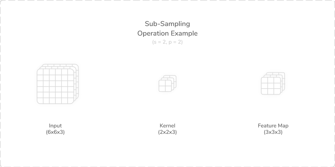
Figure 3 shows a subsampling operation that involved a 3-channel (6×6) image and a 3-channel (2×2) kernel. The operation was implemented with a stride of two and zero padding. This meant that the kernel moved over each (2×2) input section in a non-overlapping motion, shifting two places between each operation. This resulted in a 3-channel (3×3) down-sampled feature map.

图3显示了涉及3通道(6×6)图像和3通道(2×2)内核的子采样操作。 该操作以两个填充和零填充的步幅实现。 这意味着内核以非重叠运动在每个(2×2)输入部分上移动，从而在每个操作之间移动了两个位置。 这产生了一个3通道(3×3)的下采样特征图。

完全连接的层 (Fully Connected Layers)

Fully connected layers were ununique to CNNs. However, they typically were included as the last few layers of most CNNs, appearing after several convolution and subsampling operations were performed. Fully connected layers were independent neural networks that possessed one or more hidden layers. Their operations involved multiplying their inputs by trainable weight vectors, with a trainable bias sometimes summed to those results. The output of these layers was traditionally sent through activation functions, similarly to convolution layers.

完全连接的层对于CNN而言是唯一的。 但是，它们通常作为大多数CNN的最后几层包括在内，出现在执行了几次卷积和二次采样操作之后。 完全连接的层是具有一个或多个隐藏层的独立神经网络。 他们的操作涉及将他们的输入乘以可训练的权重向量，有时将可训练的偏差加到那些结果上。 这些层的输出传统上是通过激活函数发送的，类似于卷积层。

Figure 4: Fully -Connected Operation Example (image y author)

图4：完全连接的操作示例(作者)

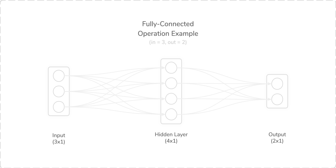
Figure 4 shows a fully connected operation that involved a (3×1) input, a (4×1) hidden layer and a (2×1) output.

图4显示了一个完全连接的操作，其中涉及一个(3×1)输入，一个(4×1)隐藏层和一个(2×1)输出。

3. LeNet-1体系结构的演练 (3. A Walkthrough of LeNet-1's Architecture)

LeNet-1 was a small CNN, which merely included five layers. The network was developed to accommodate minute, single-channel images of size (28×28). It boasted a total of 3,246 trainable parameters and 139,402 connections.

LeNet-1是一个小型CNN，仅包含五层。 开发该网络是为了容纳尺寸为(28×28)的微小单通道图像。 它总共拥有3246个可训练参数和139402个连接。

Figure 5: LeNet-1 Architecture Diagram (image by author)

图5：LeNet-1体系结构图(作者提供)

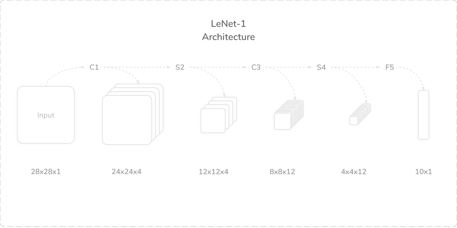
LeNet-1 was initially trained on LeCun’s [2] USPS database, where it incurred a 1.7% error rate. During this testing, the images were downsampled to a (16×16) tensor, then centred in a larger (28×28) tensor. This processing was done by using a customised input layer. The five layers of the LeNet-1 were as follows:

LeNet-1最初是在LeCun的[2] USPS数据库中进行训练的，错误率达1.7％。 在此测试过程中，将图像降采样为(16×16)张量，然后在较大的(28×28)张量中居中。 通过使用定制的输入层来完成此处理。 LeNet-1的五层如下：

1. Layer C1: Convolution Layer (num_kernels=4, kernel_size=5×5, padding=0, stride=1)
   C1层：卷积层(num_kernels = 4，kernel_size = 5×5，padding = 0，stride = 1)
2. Layer S2: Average Pooling Layer (kernel_size=2×2, padding=0, stride=2)
   S2层：平均池化层(kernel_size = 2×2，padding = 0，stride = 2)
3. Layer C3: Convolution Layer (num_kernels=12, kernel_size=5×5, padding=0, stride=1)
   C3层：卷积层(num_kernels = 12，kernel_size = 5×5，padding = 0，stride = 1)
4. Layer S4: Average Pooling Layer (kernel_size=2×2, padding=0, stride=2)
   S4层：平均池化层(kernel_size = 2×2，padding = 0，步幅= 2)
5. Layer F5: Fully Connected Layer (out_features=10)
   F5层：完全连接的层(out_features = 10)

Figure 6: LeNet-1 C1 — First Convolution Layer Diagram (image by author)

图6：LeNet-1 C1 —第一卷积层图(作者提供的图像)

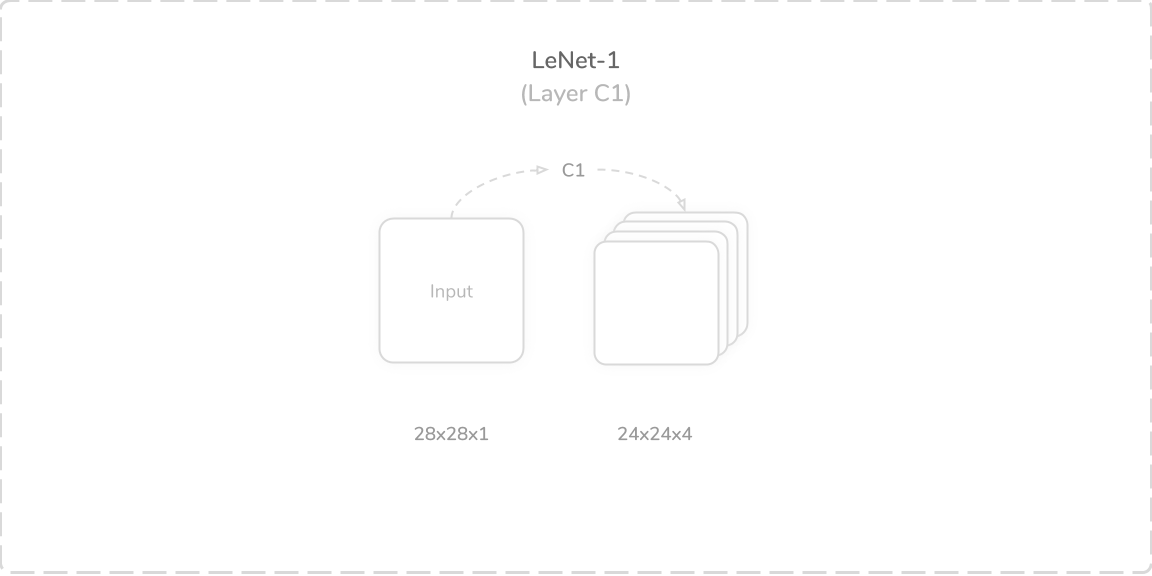
C1：第一卷积层 (C1: First Convolution Layer)

LeNet-1’s first layer was a convolutional layer that accepted a (28×28×1) image tensor as its input. It performed a zero-padded convolution operation using four (5×5) kernels with a stride of one. This produced a (24×24×4) output tensor which was passed through a hyperbolic tangent (tanh) activation function, then onto the layer S2. The tanh function, as with all activation functions present in the network, was used to introduce non-linearity. The layer had 104 trainable parameters and 59,904 connections.

LeNet-1的第一层是卷积层，它接受(28×28×1)图像张量作为输入。 它使用步幅为1的四个(5×5)内核执行了零填充卷积操作。 这产生了(24×24×4)输出张量，该张量通过双曲正切(tanh)激活函数，然后传递到层S2上。 tanh函数与网络中存在的所有激活函数一样，用于引入非线性。 该层具有104个可训练参数和59,904个连接。

Figure 7: LeNet-1 S2 — First Average Pooling Layer Diagram (image by author)

图7：LeNet-1 S2 —第一平均池化层图(作者提供的图像)

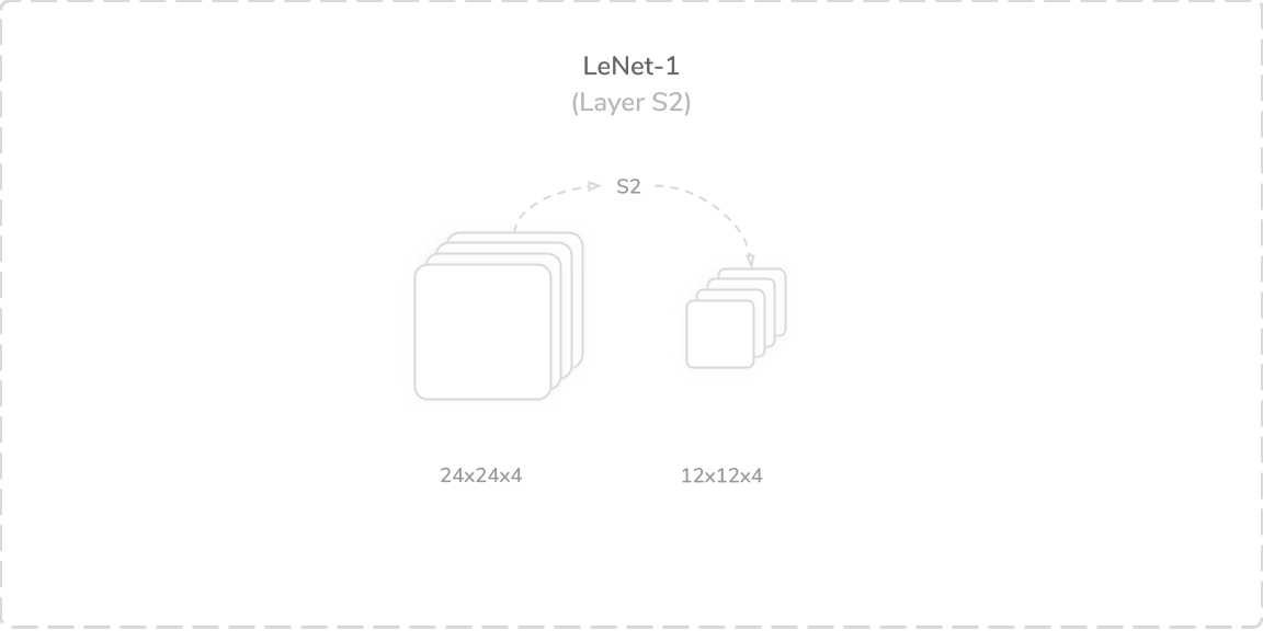
S2：第一平均池化层 (S2: First Average Pooling Layer)

LeNet-1’s second layer was an average pooling layer that accepted output from the layer C1, a (24×24×4) tensor, as its input. It performed a zero-padded subsampling operation utilising a (2×2) kernel (window region) with a stride of two. This produced a (12×12×4) output tensor that was then passed to the layer C3.

LeNet-1的第二层是平均池化层，它接受来自C1层的输出(24×24×4)张量作为其输入。 它利用步幅为2的(2×2)内核(窗口区域)执行了零填充二次采样操作。 这产生了(12×12×4)输出张量，然后将其传递到层C3。

Figure 8: LeNet-1 C3— Second Convolution Layer Diagram (image by author)

图8：LeNet-1 C3-第二卷积层图(作者提供)

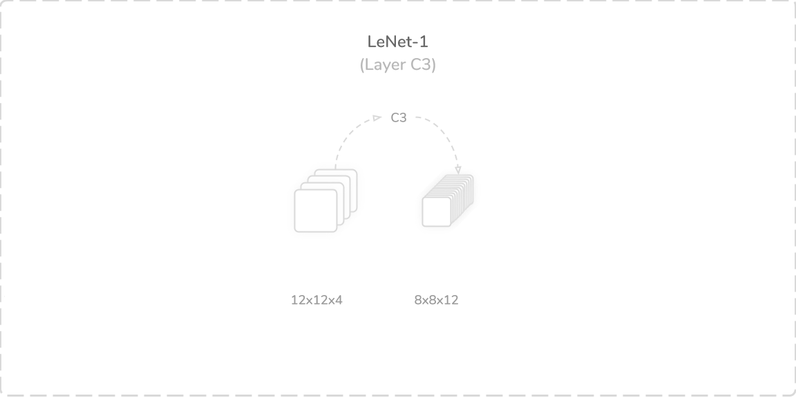
C3：第二卷积层 (C3: Second Convolution Layer)

LeNet-1’s third layer was another convolutional layer that accepted output from the layer S2, a (12×12×4) tensor, as its input. It also performed a zero-padded convolution operation; however, it alternately used twelve (5×5) kernels with a stride of one. This produced an (8×8×12) output tensor that was then passed through a tanh activation function then onto the layer S4. The layer boasted 1,212 trainable parameters and 77,568 connections, which summed to a total of 1,316 trainable parameters and 137,472 connections so far.

LeNet-1的第三层是另一个卷积层，它接受来自层S2的输出(一个12×12×4)张量作为其输入。 它还执行了零填充卷积操作； 但是，它交替使用十二个(5×5)内核，步幅为1。 这产生(8×8×12)输出张量，然后将其通过tanh激活函数传递到层S4上。 该层拥有1,212个可训练参数和77,568个连接，到目前为止，总共有1,316个可训练参数和137,472个连接。

Figure 9: LeNet-1 S4— Second Average Pooling Layer Diagram (image by author)

图9：LeNet-1 S4-第二平均池化层图(作者提供的图像)

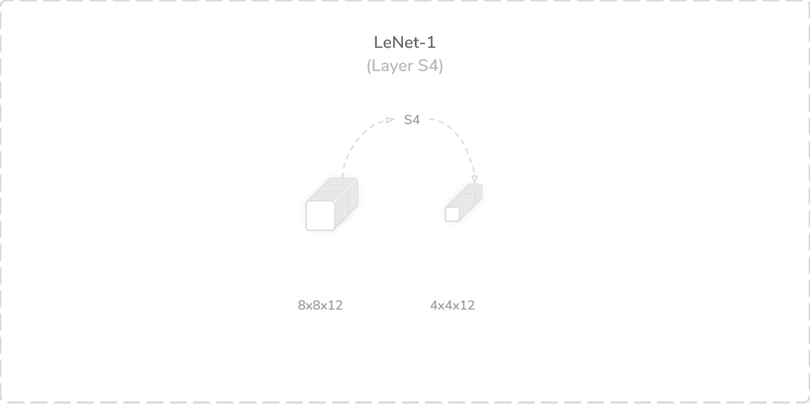
S4：第二平均池化层 (S4: Second Average Pooling Layer)

LeNet-1’s fourth layer was another average pooling layer that accepted output from the layer C3, an (8×8×12) tensor, as its input. It performed a zero-padded subsampling operation, similar to the layer S2, using a (2×2) kernel with a stride of two. This produced a (4×4×12) output tensor that was then passed onto the layer F5.

LeNet-1的第四层是另一个平均池化层，它接受来自C3层(一个8×8×12)张量的输出作为其输入。 它使用步幅为2的(2×2)内核执行了类似于S2层的零填充二次采样操作。 这产生(4×4×12)输出张量，然后将其传递到层F5上。

Figure 10: LeNet-1 F5 — Fully Connected Layer Diagram (image by author)

图10：LeNet-1 F5 —完全连接的层图(作者提供的图像)

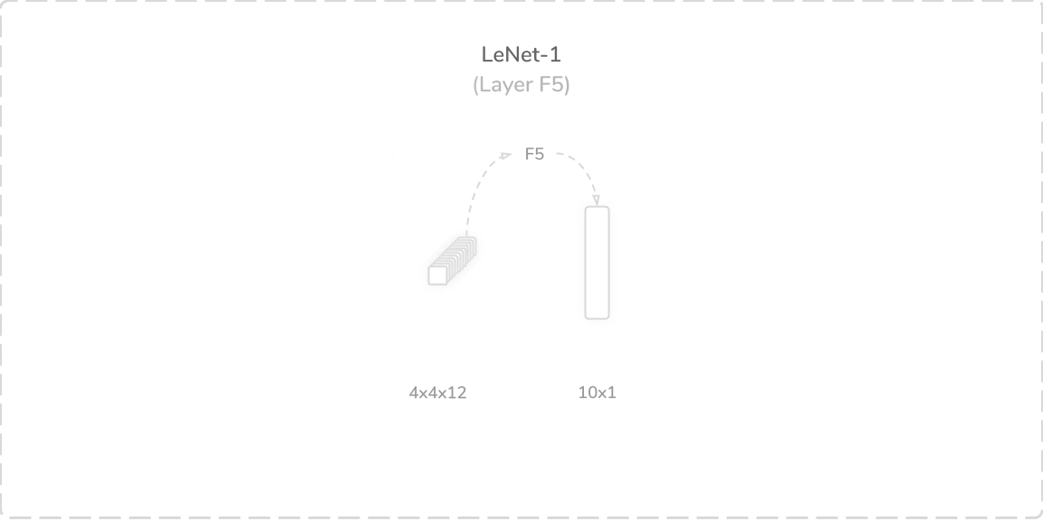
F5：完全连接的层 (F5: Fully Connected Layer)

The fifth and final layer of LeNet-1 was a fully connected (dense) layer that accepted the flattened output of the layer S4, a flattened (4×4×12) tensor, as its input. It performed a weighted sum operation with an added bias term. This produced a (10×1) output tensor that was then passed through a softmax activation function. The output of the softmax activation function contained the predictions of the network. This layer contained 1,930 trainable parameters and connections, which summed to a total of 3,246 trainable parameters and 139,402 connections overall.

LeNet-1的第五层也是最后一层是完全连接的(密集)层，该层接受层S4的平坦输出(平坦(4×4×12)张量)作为其输入。 它执行了加权和运算，并加上了偏差项。 这产生了(10×1)输出张量，然后将其通过softmax激活函数传递。 softmax激活函数的输出包含网络的预测。 该层包含1,930个可训练参数和连接，总计总计3,246个可训练参数和139,402个连接。

4. LeNet-4体系结构的演练 (4. A Walkthrough of LeNet-4’s Architecture)

LeNet-4 was a six layer CNN, which improved upon LeNet-1. The key difference between the two was an additional fully connected layer included in LeNet-4. LeNet-4 was also built to accommodate a larger image size of (32×32), compared to (24×24) for LeNet-1. The network boasted a total of 51,050 trainable parameters and 292,466 connections.

LeNet-4是一个六层的CNN，在LeNet-1的基础上进行了改进。 两者之间的主要区别在于LeNet-4中包含一个附加的完全连接层。 与LeNet-1的(24×24)相比，LeNet-4还可以容纳更大的图像尺寸(32×32)。 该网络总共拥有51,050个可训练参数和292,466个连接。

Figure 11: LeNet-4 Architecture Diagram (image by author)

图11：LeNet-4架构图(作者提供)

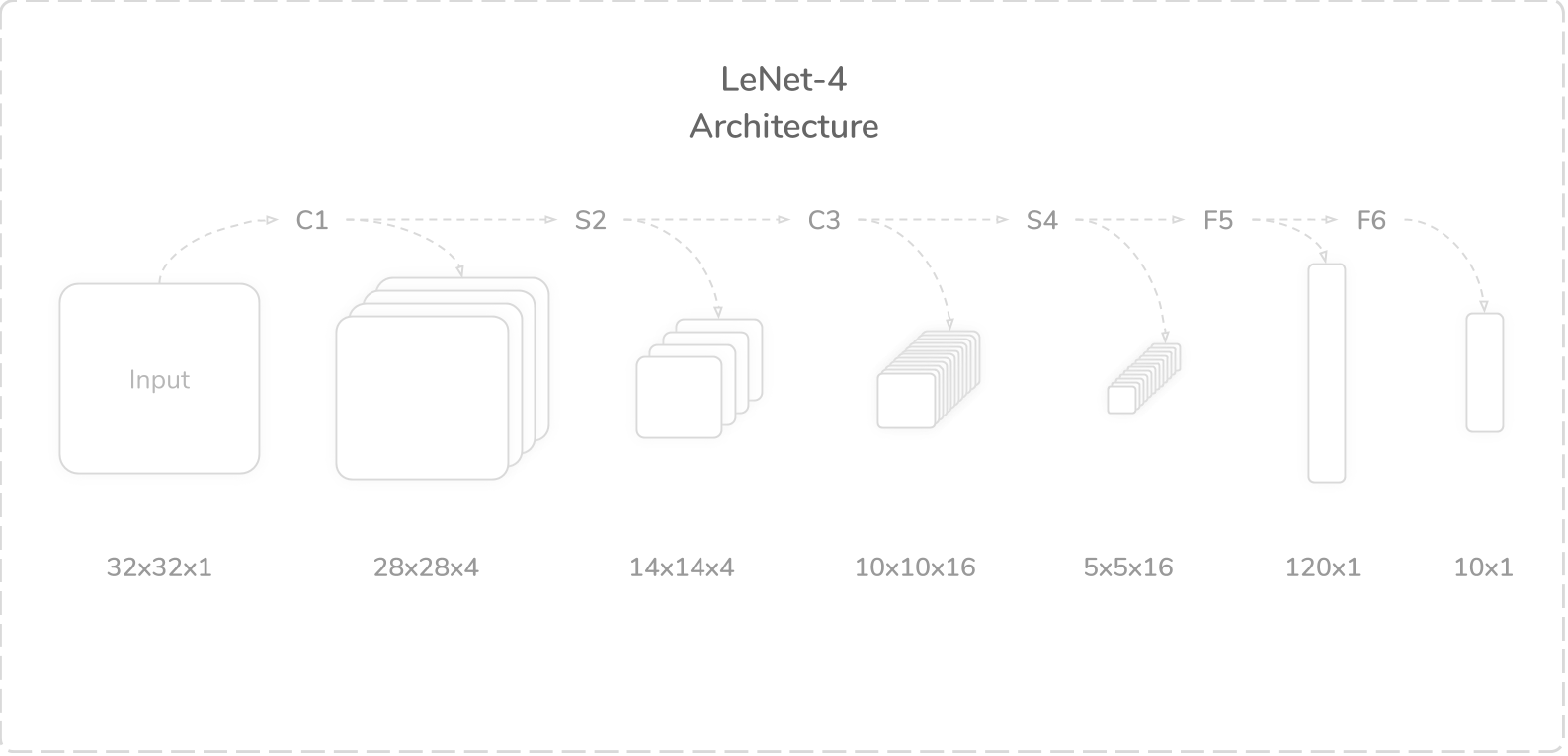
During LeNet-4's testing phase, the authors used test images that were downsampled to a (20×20) tensor and then centred into a larger (32×32) tensor. The network was established by the authors to incur a 1.1% error rate on test data, which represented a 35% decrease compared to LeNet-1. The six layers of LeNet-4 were as follows:

在LeNet-4的测试阶段，作者使用的测试图像先降采样为(20×20)张量，然后居中为更大的(32×32)张量。 作者建立了该网络，以使测试数据的错误率达到1.1％，与LeNet-1相比，降低了35％。 LeNet-4的六个层如下：

1. Layer C1: Convolution Layer (num_kernels=4, kernel_size=5×5, padding=0, stride=1)
   C1层：卷积层(num_kernels = 4，kernel_size = 5×5，padding = 0，stride = 1)
2. Layer S2: Average Pooling Layer (kernel_size=2×2, padding=0, stride=2)
   S2层：平均池化层(kernel_size = 2×2，padding = 0，stride = 2)
3. Layer C3: Convolution Layer (num_kernels=16, kernel_size=5×5, padding=0, stride=1)
   C3层：卷积层(num_kernels = 16，kernel_size = 5×5，padding = 0，stride = 1)
4. Layer S4: Average Pooling Layer (kernel_size=2×2, padding=0, stride=2)
   S4层：平均池化层(kernel_size = 2×2，padding = 0，步幅= 2)
5. Layer F5: Fully Connected Layer (out_features=120)
   F5层：完全连接的层(out_features = 120)
6. Layer F6: Fully Connected Layer (out_features=10)
   F6层：完全连接的层(out_features = 10)

Figure 12: LeNet-4 C1— First Convolution Layer Diagram (image by author)

图12：LeNet-4 C1-第一卷积层图(作者提供的图像)

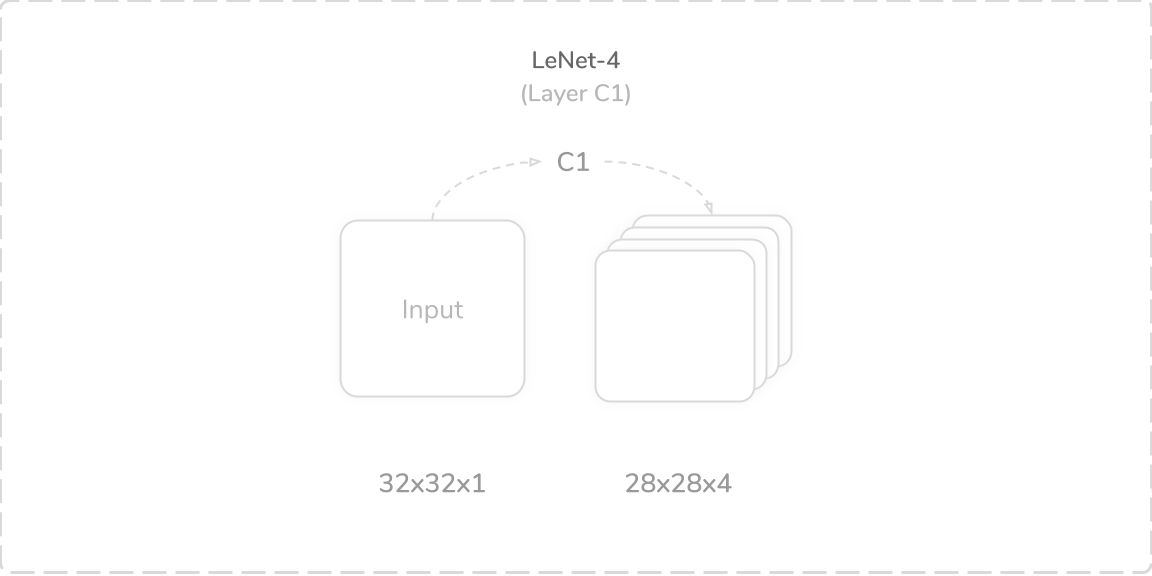
C1：第一卷积层 (C1: First Convolution Layer)

LeNet-4’s first layer was a convolutional layer that accepted a (32×32×1) image tensor as its input. It performed a zero-padded convolution operation using four (5×5) kernels with a stride of one. This produced a (28×28×4) output tensor that was then passed through a tanh activation function then onto the layer S2. The layer had 104 trainable parameters and 81,536 connections.

LeNet-4的第一层是卷积层，它接受(32×32×1)图像张量作为输入。 它使用步幅为1的四个(5×5)内核执行了零填充卷积操作。 这产生了(28×28×4)输出张量，然后将其通过tanh激活函数传递到层S2上。 该层具有104个可训练参数和81,536个连接。

Figure 13: LeNet-4 S2 — First Average Pooling Layer Diagram (image by author)

图13：LeNet-4 S2 —第一平均池化层图(作者提供的图像)

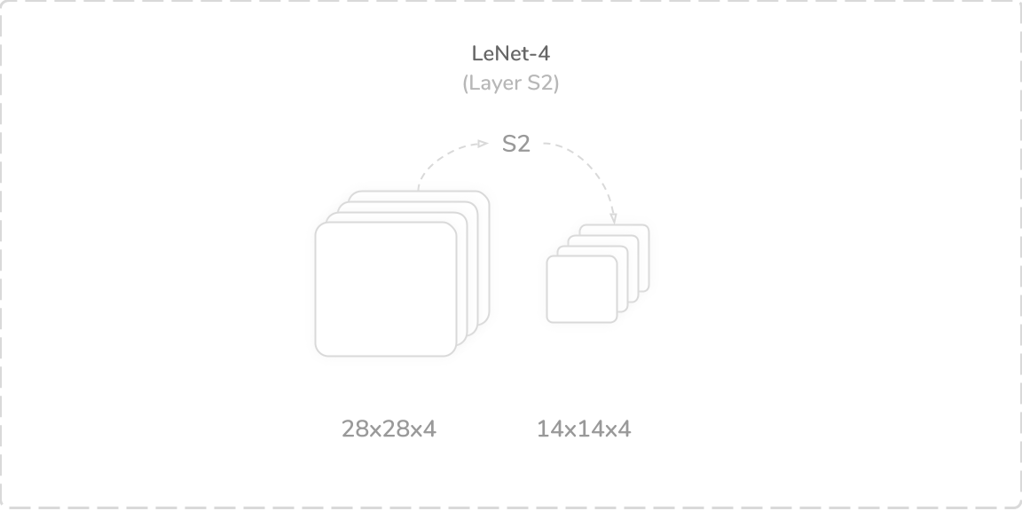
S2：第一平均池化层 (S2: First Average Pooling Layer)

LeNet-4’s second layer was an average pooling layer that accepted output from the layer C1, a (28×28×4) tensor, as its input. It performed a zero-padded subsampling operation using a (2×2) kernel with a stride of two. This produced a (14×14×4) output tensor that was then passed to the layer C3.

LeNet-4的第二层是平均池化层，它接受来自C1层(28×28×4)张量的输出作为其输入。 它使用步幅为2的(2×2)内核执行了零填充子采样操作。 这产生了(14×14×4)输出张量，然后将其传递到层C3。

Figure 14: LeNet-4 C3 — Second Convolution Layer Diagram (image by author)

图14：LeNet-4 C3-第二卷积层图(作者提供的图像)

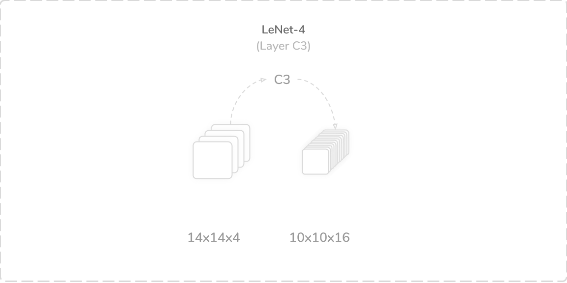
C3：第二卷积层 (C3: Second Convolution Layer)

LeNet-4’s third layer was another convolutional layer that accepted output from the layer S2, a (14×14×4) tensor, as its input. It performed the same zero-padded convolution operation as the layer C1; however, it alternately used sixteen (5×5) kernels with a stride of one. This produced a (10×10×16) output tensor that was then passed through a tanh activation function then onto the layer S4. The layer contained 1,616 trainable parameters and 161,600 connections, which summed to a total of 1,720 trainable parameters and 243,136 connections so far.

LeNet-4的第三层是另一个卷积层，它接受来自S2层的输出(14×14×4)张量作为其输入。 它执行了与C1层相同的零填充卷积操作； 但是，它轮流使用步幅为1的十六个(5×5)内核。 这产生了(10×10×16)输出张量，然后将其通过tanh激活函数传递到层S4上。 该层包含1,616个可训练参数和161,600个连接，到目前为止，总共有1,720个可训练参数和243,136个连接。

Figure 15: LeNet-4 S4 — Second Average Pooling Layer Diagram (image by author)

图15：LeNet-4 S4 —第二平均池化层图(作者提供的图像)

S4：第二平均池化层 (S4: Second Average Pooling Layer)

LeNet-4's fourth layer was another average pooling layer that accepted output from the layer C3, a (10×10×16) tensor, as its input. It performed a zero-padded subsampling operation using a (2×2) kernel with a stride of two. This produced a (5×5×16) output tensor that was then passed to the layer F5.

LeNet-4的第四层是另一个平均池化层，它接受来自C3层的输出(10×10×16)张量作为其输入。 它使用步幅为2的(2×2)内核执行了零填充子采样操作。 这产生了(5×5×16)输出张量，然后将其传递到层F5。

Figure 16: LeNet-4 F5 — First Fully Connected Layer Diagram (image by author)

图16：LeNet-4 F5 —第一个完全连接的层图(作者提供的图像)

F5：第一个完全连接的层 (F5: First Fully Connected Layer)

LeNet-4’s fifth layer was a fully connected layer that accepted the flattened output of the layer S4, a flattened (5×5×16) tensor, as its input. It performed the traditional weighted sum operation with an added bias term. This produced a (120×1) output tensor that was then passed through a tanh activation function then onto the layer F6. The layer contained 48,120 trainable parameters and connections, which summed to a total of 48,840 trainable parameters and 291,256 connections so far.

LeNet-4的第五层是完全连接的层，接受层S4的平坦输出(平坦(5×5×16)张量)作为其输入。 它执行传统的加权和运算，并增加了偏差项。 这产生了(120×1)输出张量，然后将其通过tanh激活函数传递到层F6上。 该层包含48,120个可训练参数和连接，到目前为止，总共有48,840个可训练参数和291,256个连接。

Figure 17: LeNet-4 F6 — Second Fully Connected Layer Diagram (image by author)

图17：LeNet-4 F6 —第二个全连接层图(作者提供的图片)

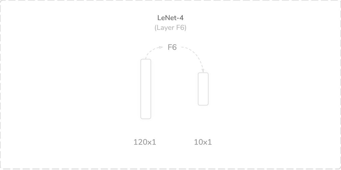
F6：第二个完全连接层 (F6: Second Fully Connected Layer)

The sixth and final layer of LeNet-4 was another fully connected layer that accepted output from the layer F5, a (120×1) tensor, as its input. It performed the traditional weighted sum operation, similarly to layer F5. This produced a (10×1) output tensor that was then passed through a softmax activation function. As with LeNet-1, the output of the softmax activation function contained the predictions of the network. The layer contained 1,210 trainable parameters and connections, which summed to a total of 51,050 trainable parameters and 292,466 connections overall.

LeNet-4的第六层也是最后一层是另一个完全连接的层，该层接受来自F5层的输出(120×1)张量作为其输入。 它执行了传统的加权和运算，类似于F5层。 这产生了(10×1)输出张量，然后将其通过softmax激活函数传递。 与LeNet-1一样，softmax激活函数的输出包含网络的预测。 该层包含1,210个可训练参数和连接，总计总计51,050个可训练参数和292,466个连接。

5. LeNet-5体系结构的演练 (5. A Walkthrough of LeNet-5’s Architecture)

The LeNet-5 network was the most popular of the three, and it represented an improvement over LeNet-4 but rather featured seven trainable layers. The network accepted a (32×32) image tensor as input and boasted a total of 60,850 trainable parameters and 340,918 connections.

LeNet-5网络是三个网络中最受欢迎的网络，它代表了对LeNet-4的改进，但具有七个可训练层。 该网络接受(32×32)图像张量作为输入，并拥有60,850个可训练参数和340,918个连接。

Figure 18: LeNet-5 Architecture Diagram (image by author)

图18：LeNet-5架构图(作者提供图片)

The LeNet-5 network was shown to incur an error rate of 0.95% on test data, which represented 44% and 13% decreases in error rates when compared to LeNet-1 and LeNet-4 respectively. The layers of the LeNet-5 architecture were as follows:

LeNet-5网络在测试数据上显示出0.95％的错误率，与LeNet-1和LeNet-4相比，其错误率分别降低了44％和13％。 LeNet-5体系结构的各层如下：

1. Layer C1: Convolution Layer (num_kernels=6, kernel_size=5×5, padding=0, stride=1)
   C1层：卷积层(num_kernels = 6，kernel_size = 5×5，padding = 0，stride = 1)
2. Layer S2: Average Pooling Layer (kernel_size=2×2, padding=0, stride=2)
   S2层：平均池化层(kernel_size = 2×2，padding = 0，stride = 2)
3. Layer C3: Convolution Layer (num_kernels=16, kernel_size=5×5, padding=0, stride=1)
   C3层：卷积层(num_kernels = 16，kernel_size = 5×5，padding = 0，stride = 1)
4. Layer S4: Average Pooling (kernel_size=2×2, padding=0, stride=2)
   S4层：平均池化(kernel_size = 2×2，padding = 0，步幅= 2)
5. Layer F5: Fully Connected Layer (out_features=140)
   F5层：完全连接的层(out_features = 140)
6. Layer F6: Fully Connected Layer (out_features=84)
   F6层：完全连接的层(out_features = 84)
7. Layer F7: Fully Connected Layer (out_features=10)
   F7层：完全连接的层(out_features = 10)

Figure 19: LeNet-5 C1— First Convolution Layer Diagram (image by author)

图19：LeNet-5 C1-第一卷积层图(作者提供的图像)

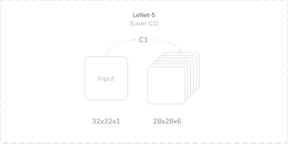
C1：第一卷积层 (C1: First Convolution Layer)

LeNet-5’s first layer was a convolutional layer that accepted a (32×32×1) image tensor as its input. It performed a zero-padded convolution operation using six (5×5) kernels with a stride of one. This produced a (28×28×6) output tensor that was then passed through a tanh activation function, then onto the layer S2. The layer contained 156 trainable parameters and 122,304 connections.

LeNet-5的第一层是卷积层，它接受(32×32×1)图像张量作为输入。 它使用步幅为1的六个(5×5)内核执行了零填充卷积运算。 这产生(28×28×6)输出张量，然后将其通过tanh激活函数，然后传递到层S2上。 该层包含156个可训练参数和122,304个连接。

Figure 20: LeNet-5 S2 — First Average Pooling Layer Diagram (image by author)

图20：LeNet-5 S2 —第一平均池化层图(作者提供的图像)

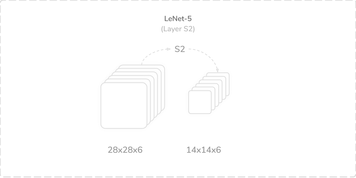
S2：第一平均池化层 (S2: First Average Pooling Layer)

LeNet-5’s second layer was an average pooling layer that accepted output from the layer C1, a (28×28×6) tensor, as its input. It performed a zero-padded subsampling operation using six (2×2) kernels with a stride of two. However, this subsampling operation multiplied the average of the regions with trainable coefficients and added trainable biases to their results. This produced a (14×14×6) output tensor that was then passed through a sigmoid activation function then onto the layer C3. The layer contained 12 trainable parameters and 5,880 connections, which summed to a total of 168 trainable parameters and 128,184 connections so far.

LeNet-5的第二层是平均池化层，它接受来自C1层(28×28×6)张量的输出作为其输入。 它使用步幅为2的六个(2×2)内核执行了零填充子采样操作。 但是，该二次采样操作将区域的平均值乘以可训练的系数，并为其结果增加了可训练的偏差。 这产生(14×14×6)输出张量，然后将其通过S型激活函数，然后传递到层C3上。 该层包含12个可训练参数和5,880个连接，到目前为止，总共有168个可训练参数和128,184个连接。

Figure 21: LeNet-5 C3 — Second Convolution Layer Diagram (image by author)

图21：LeNet-5 C3 —第二卷积层图(作者提供的图像)

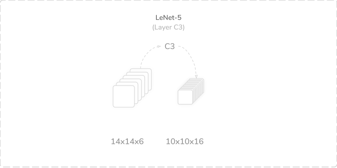
C3：第二卷积层 (C3: Second Convolution Layer)

LeNet-5’s third layer was another convolutional layer that accepted output from the layer S2, a (14×14×6) tensor, as its input. However, it performed a zero-padded convolution operation using sixteen (5×5) kernels instead of six, along with a stride of one. The operation also only used a subset of the prior the layer S2’s feature maps. This produced a (10×10×16) output tensor that was then passed through a tanh activation function then onto the layer S4. The layer contained 1,516 trainable parameters and 151,600 connections, which summed to a total of 1,684 trainable parameters and 279,784 connections so far.

LeNet-5的第三层是另一个卷积层，它接受来自S2层的输出(14×14×6)张量作为其输入。 但是，它使用十六(5×5)个内核而不是六个内核执行了零填充卷积运算，步幅为一。 该操作还仅使用了层S2的特征图之前的子集。 这产生了(10×10×16)输出张量，然后将其通过tanh激活函数传递到层S4上。 该层包含1,516个可训练参数和151,600个连接，到目前为止，总共有1,684个可训练参数和279,784个连接。

Figure 22: LeNet-5 S4 — Second Average Pooling Layer Diagram (image by author)

图22：LeNet-5 S4 —第二平均池化层图(作者提供的图像)

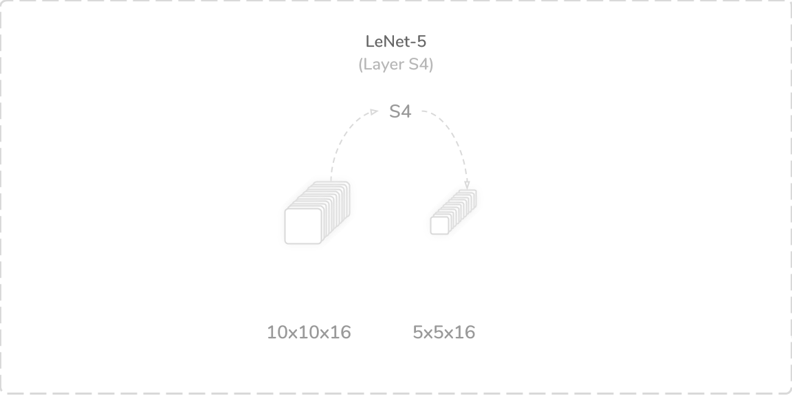
S4：第二平均池化层 (S4: Second Average Pooling Layer)

LeNet-5’s fourth layer was another average pooling layer that accepted output from the layer C3, a (10×10×16) tensor, as its input. It performed a zero-padded subsampling operation using a (2×2) kernel with a stride of two. The subsampling operation operated the same as in the layer S2. This produced a (5×5×16) output tensor that was then passed through a sigmoid activation function then onto the layer F5. The layer contained 32 trainable parameters and 2,000 connections, which summed to a total of 1,716 trainable parameters and 281,784 connections so far.

LeNet-5的第四层是另一个平均池化层，它接受来自C3层的输出(10×10×16)张量作为其输入。 它使用步幅为2的(2×2)内核执行了零填充子采样操作。 二次采样操作与层S2中的操作相同。 这产生了(5×5×16)输出张量，然后将其通过S型激活函数，然后传递到层F5上。 该层包含32个可训练参数和2,000个连接，到目前为止，总共有1,716个可训练参数和281,784个连接。

Figure 23: LeNet-5 F5 — First Fully Connected Layer Diagram (image by author)

图23：LeNet-5 F5 —第一个完全连接的层图(作者提供的图像)

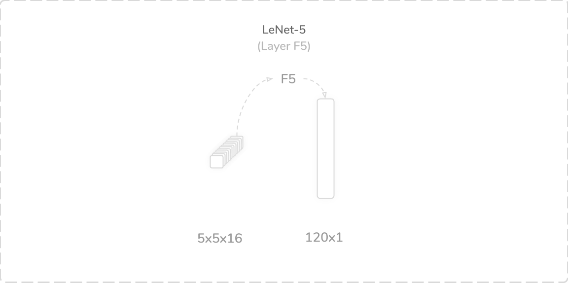
F5：第一个完全连接的层 (F5: First Fully Connected Layer)

LeNet-5’s fifth layer was a fully connected layer that accepted the flattened output from the layer S4, a flattened (5×5×16) tensor, as its input. It performed the traditional weighted sum operation with an added bias term. This produced a (120×1) output tensor that was then passed through a tanh activation function then onto the layer F6. The layer contained 48,120 trainable parameters and connections, which summed to a total of 49,836 trainable parameters and 329,904 connections so far.

LeNet-5的第五层是完全连接的层，该层接受来自层S4的平坦输出(平坦(5×5×16)张量)作为其输入。 它执行传统的加权和运算，并增加了偏差项。 这产生了(120×1)输出张量，然后将其通过tanh激活函数传递到层F6上。 该层包含48,120个可训练参数和连接，到目前为止，总共有49,836个可训练参数和329,904个连接。

Figure 24: LeNet-5 F6 — Second Fully Connected Layer Diagram (image by author)

图24：LeNet-5 F6 —第二个全连接层图(作者提供的图像)

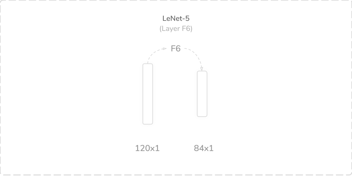
F6：第二个完全连接层 (F6: Second Fully Connected Layer)

LeNet-5’s sixth layer was another fully connected layer that accepted output from the layer F5, a (120×1) tensor, as its input. It performed the same operation as layer F5 and produced an (84×1) output tensor that was then passed through a tanh activation function then onto the layer F7. The layer contained 10,164 trainable parameters and connections, which summed to a total of 60,000 trainable parameters and 340,068 connections so far.

LeNet-5的第六层是另一个完全连接的层，该层接受来自F5层的输出(120×1)张量作为其输入。 它执行与F5层相同的操作，并产生(84×1)输出张量，然后将其通过tanh激活函数传递到F7层上。 该层包含10,164个可训练的参数和连接，到目前为止，总共有60,000个可训练的参数和340,068个连接。

Figure 25: LeNet-5 F7 — Third Fully Connected Layer Diagram (image by author)

图25：LeNet-5 F7 —第三层完全连接的层图(作者提供的图像)

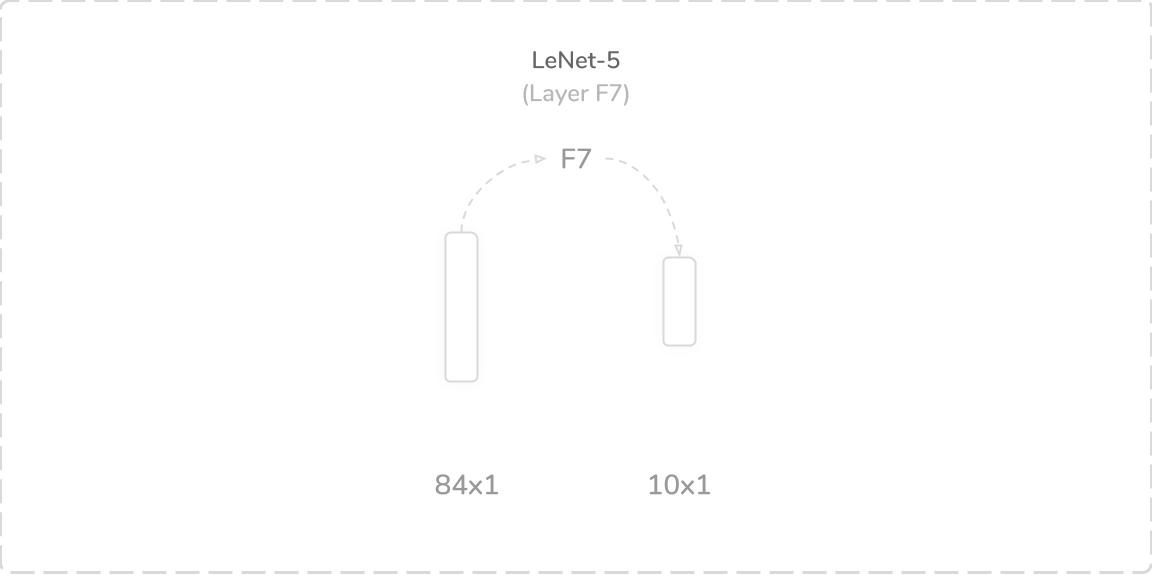
F7：第三层完全连接层 (F7: Third Fully Connected Layer)

The seventh and final layer of LeNet-5 was another fully connected layer that accepted output from the layer F6, an (84×1) tensor, as its input. It performed the same operation as layers F5 and F6 and produced a (10×1) output tensor that was then passed through a softmax activation function. As with LeNet-1 and LeNet-4, the output of the softmax activation function contained the predictions of the network. The layer contained 850 trainable parameters and connections, which summed to a total of 60,850 trainable parameters and 340,918 connections overall.

LeNet-5的第七层也是最后一层是另一个完全连接的层，该层接受来自F6层(一个84×1)张量的输出作为其输入。 它执行与层F5和F6相同的操作，并生成(10×1)输出张量，然后将其通过softmax激活函数。 与LeNet-1和LeNet-4一样，softmax激活函数的输出包含网络的预测。 该层包含850个可训练参数和连接，总计总计60,850个可训练参数和340,918个连接。

6. LeNet分析 (6. Analysis of LeNet)

LeNet-1 was trained on LeCun’s USPS dataset. Whereas LeNet-4 and LeNet-5 were trained on the MNIST dataset. All LeNet variants were commonly trained using Maximum Likelihood Estimation (MLE) and Mean Squared Error (MSE) loss. The input images for LeNet were normalised such that their values remain within the range [-0.1, 1.175], which made the mean 0 and the variance roughly 1. It was argued that normalisation accelerated the network’s learning. While the LeNet CNNs marked a breakthrough for their time, there were several limitations:

LeNet-1在LeCun的USPS数据集上进行了培训。 而LeNet-4和LeNet-5在MNIST数据集上进行了训练。 通常使用最大似然估计(MLE)和均方误差(MSE)损失来训练所有LeNet变体。 对LeNet的输入图像进行了归一化处理，以使其值保持在[-0.1，1.175]范围内，这使得平均值为0，方差大致为1。有人认为归一化可以加速网络的学习。 LeNet CNN在其时代上取得了突破，但存在一些局限性：

1. The networks were small and therefore had limited applications where they worked correctly.
   该网络很小，因此在正常工作的应用程序中受到限制。
2. The networks only worked with single-channel (black and white images), which also limited its applications.
   这些网络仅适用于单通道(黑白图像)，这也限制了其应用。
3. Most modern adaptations of this model implement a max-pooling operation as opposed to an average pooling operation as it allows for more rapid convergence due to the larger gradients returned during back-propagation.
   该模型的大多数现代改型都实现了最大池化操作，而不是平均池化操作，因为由于反向传播过程中返回的较大梯度，它允许更快的收敛。
4. Most modern adaptations implement a ReLu activation as opposed to tanh and sigmoid as ReLu usually leads to higher classification accuracies.
   大多数现代改编都实现了ReLu激活，而与tanh和Sigmoid相反，因为ReLu通常会导致更高的分类精度。

7. LeNet的摘要 (7. Summary of LeNet)

To summarise, the following represent some key takeaways about the LeNet networks:

总而言之，以下内容代表了有关LeNet网络的一些关键要点：

1. Operated with single-channel images, either (28×28) or (32×32) in size.
   使用大小为(28×28)或(32×32)的单通道图像进行操作。
2. Used tanh activation functions as opposed to ReLu.
   与ReLu相反，使用了tanh激活功能。
3. Used average pooling as opposed to max pooling for subsampling.
   使用平均池而不是最大池进行二次采样。
4. Used (2×2) kernels for average pooling subsampling.
   使用(2×2)个内核进行平均池子采样。
5. Used (5×5) kernels for convolutions.
   使用(5×5)内核进行卷积。
6. Trained by optimising for Mean Squared Error (MSE) loss.
   通过优化均方误差(MSE)损失进行培训。
7. Included trainable coefficient and bias for some subsampling operations.
   包括一些子采样操作的可训练系数和偏差。
8. Classified images into one of ten classes.
   将图像分类为十个类别之一。

下一步 (Next Steps)

Now that you possess this knowledge about the LeNet networks, you can utilize prebuilt LeNet models or even implement one yourself with libraries like PyTorch or Keras. Keep in mind the limitations of LeNet, and you should achieve decent results by training it yourself with the MNIST dataset.

现在，你拥有这方面的知识对LeNet网络，您可以使用预置的LeNet机型甚至自己实现一个与像库PyTorch或Keras 。 请记住LeNet的局限性，您应该通过使用MNIST数据集自己对其进行训练来获得不错的结果。

翻译自: https://towardsdatascience.com/understanding-lenet-a-detailed-walkthrough-17833d4bd155

攻防演练