在流中抛出张量_在张量流中实现胶囊网络

在流中抛出张量

We are well aware that Convolution Neural Network(CNN) has outperformed humans in many computer vision tasks. All the CNN based models have the same base architecture of the Convolution layer followed by Pooling layers with intermediate Batch Normalization layers, for normalizing batch in the forward pass and controlling the gradients in the backward pass.

我们很清楚，在许多计算机视觉任务中，卷积神经网络(CNN)的性能均优于人类。 所有基于CNN的模型都具有与卷积层相同的基本体系结构，其后是具有中间批处理归一化层的池化层，用于在前向遍历中归一化批次并在后向遍历中控制梯度。

However, there were a couple of drawbacks in CNN primarily the Max Pooling layer as it does not consider the relation between pixel having maximum value and its immediate neighbors. To solve the problem, Hinton comes up with the idea of Capsule Network and an algorithm called “Dynamic Routing Between Capsules”. Many resources have explained the intuition and the architecture of the model. You can have a look at them in the series of blog posts here.

但是，在CNN中，主要是最大池化层有几个缺点，因为它没有考虑具有最大值的像素与其直接相邻像素之间的关系。 为了解决该问题，Hinton提出了胶囊网络的思想和一种称为“ 胶囊之间动态路由 ”的算法。 许多资源已经说明了模型的直觉和体系结构。 您可以在此处的一系列博客文章中查看它们 。

In this post, I have explained the implementation details of the model. It assumes a good understanding of Tensors and TensorFlow Custom Layers and Models.

在这篇文章中，我已经解释了该模型的实现细节。 假定您对Tensor和TensorFlow 自定义层和模型有很好的了解。

This post has been structured as follows:

帖子的结构如下：

• Essential TensorFlow Operations
  TensorFlow基本操作
• Capsule Layer Class
  胶囊层类
• Miscellaneous Details
  杂项详细信息
• Results and Feature Visualization
  结果和特征可视化

TensorFlow操作 (TensorFlow Operations)

Building a model in TensorFlow 2.3 with a Functional API or Sequential model is quite easy with very few lines of code. However, in this capsule network implementation, we make use of Functional API as well as some custom operations and decorated them with the @tf.function for optimization. In this section, I am just going to highlight the tf.matmul function for higher dimensions. If you are familiar with this, then you can skip this section and move ahead to the next one.

使用功能性API或顺序模型在TensorFlow 2.3中构建模型非常简单，只需很少的代码行。 但是，在此胶囊网络的实现中，我们利用Functional API以及一些自定义操作，并使用@tf.function装饰它们以进行优化。 在本节中，我将重点介绍tf.matmul函数以实现更大的尺寸。 如果您对此很熟悉，则可以跳过本节，然后继续进行下一部分。

tf.matmul (tf.matmul)

For 2D Matrices, the matmul operation performs matrix multiplication operations provided the shape signatures are respected. However, for tensors with rank (r > 2), the operation becomes a combination of 2 operations i.e., element-wise multiplication and matrix multiplication.

对于2D矩阵，只要遵守形状签名，matmul操作即可执行矩阵乘法操作。 但是，对于秩为(r> 2)的张量，该运算将成为2个运算的组合，即逐元素乘法和矩阵乘法。

For a rank (r = 4) matrices, it first performs broadcasting along the axis = [0, 1] and makes each of them of equal shape. And the last two axes ([2,3]) undergo matrix multiplication if and only if the last dimension of the first tensor and the second to last dimension of the second tensor should have the matching dimensions. The example below will explain it, for brevity I have only printed the shapes, but feel free to print and calculate the number on the console.

对于秩(r = 4)的矩阵，它首先沿轴= [0，1]进行广播 ，并使它们的形状相同。 并且仅当第一个张量的最后一个维度和第二个张量的第二个至最后一个维度具有匹配的维度时，最后两个轴([2,3])才会进行矩阵乘法。 为了简洁起见，下面的示例将对其进行说明，为简便起见，我仅打印形状，但可以在控制台上随意打印并计算数字。

>>> w = tf.reshape(tf.range(48), (1,8,3,2))
>>> x = tf.reshape(tf.range(40), (5,1,2,4))
>>> tf.matmul(w, x).shape
TensorShape([5, 8, 3, 4])

w is broadcasted along axis=0 and x is broadcasted along axis=1, and the remaining two dimensions were matrix multiplied. Let’s check out the transpose_a/transpose_b parameter of matmul. On calling tf.transpose on a tensor all the dimensions are reversed. For example,

w沿轴= 0广播，x沿轴= 1广播，其余两个维度矩阵相乘。 让我们检查一下matmul的transpose_a / transpose_b参数。 在张量上调用tf.transpose时，所有尺寸都将反转。 例如，

>>> a = tf.reshape(tf.range(48), (1,8,3,2))
>>> tf.transpose(a).shape
TensorShape([2, 3, 8, 1])

So let’s just see how it work in tf.matmul

因此，让我们看看它在tf.matmul如何工作

>>> w = tf.ones((1,10,16,1))
>>> x = tf.ones((1152,1,16,1))
>>> tf.matmul(w, x, transpose_a=True).shape
TensorShape([1152, 10, 1, 1])

Wait !!! I was expecting an error but it worked out fine. How ???

等等!!! 我期待一个错误，但是效果很好。 怎么样 ？？？

What TensorFlow did was first it broadcasted along the first two dimensions and then assumed them as a stack of 2D matrices. You could visualize it as transposed being applied only to the last two dimensions, of the first array. The shape of the first array after the transpose operation was [1152, 10, 1, 16] (Transpose applied to the last two-dimension), and now matrix multiplication is applied. By the way, transpose_a = True means the above-mentioned transpose operation will be applied to the first element provided in matmul. Refer to the docs for more details.

TensorFlow所做的工作首先是沿前两个维度广播，然后将它们假定为2D矩阵堆栈。 您可以将其可视化为仅应用于第一个数组的最后两个维度的转置。 转置操作后的第一个数组的形状为[1152、10、1、16](将转置应用于最后一个二维)，现在应用矩阵乘法。 顺便说一下， transpose_a = True意味着上述转置操作将应用于matmul中提供的第一个元素。 有关更多详细信息，请参考文档。

Okay!! That’s enough to get through this post. We can now check out the code for Capsule Layer.

好的！！ 这足以完成这篇文章。 现在，我们可以签出Capsule Layer的代码。

胶囊层类 (Capsule Layer Class)

Let’s see what’s happening in the code.

让我们看看代码中发生了什么。

Note: All the hyper-parameters are used the same as that from the paper.

注意：所有超参数的使用与本文中的相同。

convolution = tf.keras.layers.Conv2D(256, [9,9], strides=[1,1], name='ConvolutionLayer', activation='relu')
primary_capsule = tf.keras.layers.Conv2D(32 * 8, [9,9], strides=[2,2], name="PrimaryCapsule")


x = self.convolution(input_x) # x.shape: (None, 20, 20, 256)
x = self.primary_capsule(x) # x.shape: (None, 6, 6, 256)

We have used tf.keras functional API to create the primary capsule outputs. These will just perform simple convolution operation in the forward pass of input image input_x. Till now we have achieved 256 (32 * 8) features maps, each of 6 x 6 size.

我们使用了tf.keras功能API来创建主要的胶囊输出。 这些将仅在输入图像input_x的正向传递中执行简单的卷积操作。 到现在为止，我们已经实现了256(32 * 8)个特征图，每个特征图的大小为6 x 6。

Now instead of visualizing the above feature map as convolution output, we re-imagine them as 32- 6 x 6 x 8 vectors piled along the last axis. Hence, we could easily obtain 6 * 6 * 32 = 1125, 8D vectors just by reshaping them. Each of these vectors is multiplied by a weight matrix which encapsulates the relation between these lower level features and the higher-level features. The dimension of the output features in the Primary Capsule Layer is 8D, and that input to the Digit Caps layer is 16D. So basically we have to multiply them with a 16 X 8 matrix. Okay, that was easy !! But wait, there are 1152 vectors in the Primary Capsule, which implies we will have 1152–16 x 8 matrices.

现在，不是将上述特征图可视化为卷积输出，而是将它们重新想象为沿最后一个轴堆积的32-6 x 6 x 8个向量。 因此，我们只需重整形状就可以轻松获得6 * 6 * 32 = 1125，8D向量。 这些向量中的每一个都与权重矩阵相乘，该权重矩阵封装了这些较低层特征和较高层特征之间的关系。 Primary Capsule层中输出要素的尺寸为8D，而Digit Caps层中的输入要素的尺寸为16D。 因此，基本上我们必须将它们与16 X 8矩阵相乘。 好吧，那很容易！ 但是，等等，主胶囊中有1152个向量，这意味着我们将拥有1152–16 x 8个矩阵。

So are we cool now ?? Nope, you forgot the number of Digits Capsule

那么，我们现在很酷吗？ 不，您忘记了数字胶囊的数量

We have 10 Digit Capsules in the next layer, and hence we will have 10 such 1152–16 x 8 matrices. So basically we get a weight tensor of shape [1152, 10,16, 8]. Each of the 1152–8D vectors of primary capsule output is contributing to each of the 10 Digit Capsules, so we could simply use the same 8D vector for each capsule in the Digit Capsule Layer. More simply we could just add a 2 new axis in 1152, 8D vectors thus converting them into the shape of [1152, 1, 8, 1]. Okay! I see what you did there, you are going to the broadcasting in tf.matmul you described above.

在下一层中，我们有10个数字胶囊，因此，我们将有10个这样的1152–16 x 8矩阵。 因此，基本上我们得到了形状为[1152，10,16，8]的重量张量。 主胶囊输出的1152-8D向量中的每一个都对10位数字胶囊中的每一个都有贡献，因此我们可以简单地对数字胶囊层中的每个胶囊使用相同的8D向量。 更简单地说，我们可以在1152个8D向量中添加2个新轴，从而将它们转换为[1152、1、8、1]的形状。 好的！ 我看到了您在这里所做的事情，您将通过上述tf.matmul进行广播。

Great !! That’s correct.

太好了！ 没错

w = tf.Variable(tf.random_normal_initializer()(shape=[1, 1152, 10, 16, 8]), dtype=tf.float32, name="Pose_Estimation")


u = tf.reshape(x, (-1, 1152, 8))
u = tf.expand_dims(u, axis=-2) # u.shape: (None, 1152, 1, 8)
u = tf.expand_dims(u,axis=-1) # # u.shape: (None, 1152, 1, 8, 1)
# In the matrix multiplication: (1, 1152, 10, 16, 8) x (None, 1152, 1, 8, 1) -> (None, 1152, 10, 16, 1)
u_hat = tf.matmul(w, u) # u_hat.shape: (None, 1152, 10, 16, 1)

Note: The shape of variable W has an extra dimension of 1 along the first axis since then the same weight has to be broadcasted for the entire batch.

注意 ：变量W的形状沿第一个轴的额外尺寸为1，因为这样一来，整个批次必须广播相同的权重。

In the u_hat, the last dimension is extraneous and was added for the correctness of matrix multiplication and hence can be now be removed using the squeeze function. The (None) in the above shapes is for the batch_size which is determined at training time.

在u_hat ，最后一个维度是多余的，为矩阵乘法的正确性添加了最后一个维度，因此现在可以使用squeeze函数将其删除。 以上形状中的(无)表示在训练时确定的batch_size 。

u_hat = tf.squeeze(u_hat, [4]) # u_hat.shape: (None, 1152, 10, 16)

Let’s move to the next step.

让我们继续下一步。

Dynamic Routing — This is where the magic begins!

动态路由-这就是魔术的开始！

paper 纸

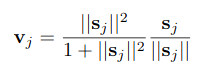
Before exploring the algorithm let’s just make the squash function and keep it for further use. I have added a small value of epsilon to avoid the gradients from exploding in-case if the denominator sums up to zero.

在探索算法之前，让我们先制作壁球功能并保留以备将来使用。 如果分母的总和为零，我添加了一个小值的epsilon，以防止梯度爆炸。

epsilon = 1e-7
def squash(self, s):
  s_norm = tf.norm(s, axis=-1, keepdims=True)
  return tf.square(s_norm)/(1 + tf.square(s_norm)) * s/(s_norm + epsilon)

In this step, the input to the Digit Capsule is the 16D vector ( u_hat ) and the no of routing iterations (r = 3) is used as specified by the paper.

在此步骤中，Digit Capsule的输入是16D向量( u_hat )，并且按照论文中的说明使用了路由迭代次数(r = 3)。

paper 纸上的路由算法

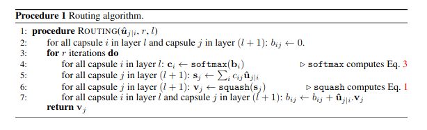
There is not much tweaking in the dynamic routing algorithm, and the code is pretty much a direct implementation of the algorithm in the paper. Have a look at the snippet below.

动态路由算法没有太多调整，并且代码几乎是本文中算法的直接实现。 看看下面的代码片段。

b = tf.zeros((input_x.shape[0], 1152, 10, 1))
for i in range(r):  
  c = tf.nn.softmax(b, axis=-2) # c.shape: (None, 1152, 10, 1)
  s = tf.reduce_sum(tf.multiply(c, u_hat), axis=1, keepdims=True) # s.shape: (None, 1, 10, 16)
  v = squash(s) # v.shape: (None, 1, 10, 16)
  agreement = tf.squeeze(tf.matmul(tf.expand_dims(u_hat, axis=-1), tf.expand_dims(v, axis=-1), transpose_a=True), [4]) # agreement.shape: (None, 1152, 10, 1)
  # Before matmul following intermediate shapes are present, they are not assigned to a variable but just for understanding the code.
  # u_hat.shape (Intermediate shape) : (None, 1152, 10, 16, 1)
  # v.shape (Intermediate shape): (None, 1, 10, 16, 1)
  # Since the first parameter of matmul is to be transposed its shape becomes:(None, 1152, 10, 1, 16)
  # Now matmul is performed in the last two dimensions, and others are broadcasted
  # Before squeezing we have an intermediate shape of (None, 1152, 10, 1, 1)
  b += agreement

Some key points should be highlighted.

一些重点应突出显示。

• The c represents the probability distribution of u_hat values and for a particular capsule in the primary capsule layer, it sums to 1. Simply speaking, the values of u_hat are distributed among the Digit capsule based on the variable c which is trained in the routing algorithm.

  c表示u_hat值的概率分布，对于主胶囊层中的特定胶囊，其总和为1。简单地说，基于路由算法训练的变量c， u_hat的值分布在Digit胶囊中。

• The Σcij ûj|i is the weighted summation of all the lower level vector which are input to the digit capsule. Since there are 1152 lower level vectors, the reduce_sum function is applied across that dimension. Setting the keep_dims=True, just makes the further computation easier.

  ∑cijûj| i是输入到数字胶囊的所有下层矢量的加权总和。 由于存在1152个较低级别的向量，因此reduce_sum函数将应用到该维度。 设置keep_dims=True ，只会使进一步的计算更加容易。

• The squash non-linearity is applied across the 16D vector of Digit Capsule to normalize the values.
  壁球非线性将应用于Digit Capsule的16D向量，以将值归一化。

• The next step has a subtle implementation where the dot product between the input and output of the digit capsule layers is calculated. This dot product governs the “agreement” between lower and higher-level capsules. You can understand the reasoning and intuition behind this step here.

  下一步是一个微妙的实现，在该实现中，将计算数字囊层的输入和输出之间的点积。 这种点积决定了低级和高级级胶囊之间的“协议”。 您可以在此处了解此步骤背后的原因和直觉。

The above loop is iterated 3 times and the hence obtained values of v are then used in the reconstruction network.

重复上述循环3次，然后将由此获得的v值用于重建网络。

Wow !! Great. You have just completed most of the difficult part. Now, it’s relatively simple.

哇 ！！ 大。 您刚刚完成了大部分困难的部分。 现在，它相对简单。

重建网络 (Reconstruction Network)

The Reconstruction network is a kind of regularizer that regenerates the images from the features of Digit Capsule Layers. While back-propagation it has an impact on the entire network, thus making features good for both prediction as well as regeneration. During training, the model uses the actual label of the input image to mask the digit caps values to zeros except the one corresponding to the label (shown in the figure below).

重建网络是一种可从Digit Capsule Layers的特征再生图像的正则化器。 在反向传播时，它会影响整个网络，因此使功能既适合预测又适合再生。 在训练期间，模型使用输入图像的实际标签将数字上限的值屏蔽为零(与标签相对应的数字除外)(如下图所示)。

the paper 纸上重建网络

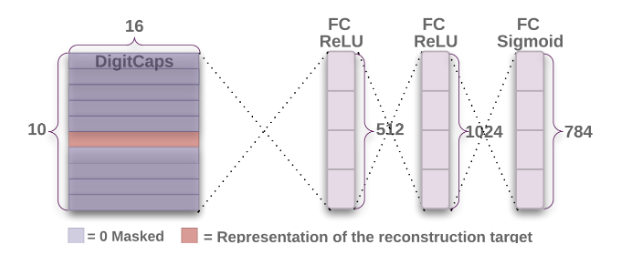
The v tensor from the above network is of shape (None, 1, 10, 16) and we broadcast and label along the 16D vector of the Digit Caps layer, and apply the masking.

来自上述网络的v张量的形状为(None，1，10，16)，我们沿Digit Caps图层的16D矢量广播和标记，并应用遮罩。

Note: One hot encoded label is used for masking.

注意 ：一个热编码标签用于遮罩。

y = tf.expand_dims(y, axis=-1) # y.shape: (None, 10, 1)
y = tf.expand_dims(y, axis=1) # y.shape: (None, 1, 10, 1)
mask = tf.cast(y, dtype=tf.float32) # mask.shape: (None, 1, 10, 1)
v_masked = tf.multiply(mask, v) # v_masked.shape: (None, 1, 10, 16)

This v_masked is then sent to the reconstruction network and which is used for regeneration of the entire image. The reconstruction network is just 3 Dense layer shown in the gist below

然后将这个v_masked发送到重建网络，并用于重建整个图像。 重建网络只是下面要点中显示的3个密集层

dense_1 = tf.keras.layers.Dense(units = 512, activation='relu')
dense_2 = tf.keras.layers.Dense(units = 1024, activation='relu')
dense_3 = tf.keras.layers.Dense(units = 784, activation='sigmoid', dtype='float32')


v_ = tf.reshape(v_masked, [-1, 10 * 16]) # v_.shape: (None, 160)
reconstructed_image = dense_1(v_) # reconstructed_image.shape: (None, 512)
reconstructed_image = dense_2(reconstructed_image) # reconstructed_image.shape: (None, 1024)
reconstructed_image = dense_3(reconstructed_image) # reconstructed_image.shape: (None, 784)

We will convert the same above code into a CapsuleNetwork Class which inherits from tf.keras.Model. You could directly use the class with your custom training loop and for prediction.

我们将上面相同的代码转换为从tf.keras.Model继承的CapsuleNetwork类。 您可以直接在自定义训练循环中使用该课程并进行预测。

class CapsuleNetwork(tf.keras.Model):
    def __init__(self, no_of_conv_kernels, no_of_primary_capsules, primary_capsule_vector, no_of_secondary_capsules, secondary_capsule_vector, r):
        super(CapsuleNetwork, self).__init__()
        self.no_of_conv_kernels = no_of_conv_kernels
        self.no_of_primary_capsules = no_of_primary_capsules
        self.primary_capsule_vector = primary_capsule_vector
        self.no_of_secondary_capsules = no_of_secondary_capsules
        self.secondary_capsule_vector = secondary_capsule_vector
        self.r = r
        
        
        with tf.name_scope("Variables") as scope:
            self.convolution = tf.keras.layers.Conv2D(self.no_of_conv_kernels, [9,9], strides=[1,1], name='ConvolutionLayer', activation='relu')
            self.primary_capsule = tf.keras.layers.Conv2D(self.no_of_primary_capsules * self.primary_capsule_vector, [9,9], strides=[2,2], name="PrimaryCapsule")
            self.w = tf.Variable(tf.random_normal_initializer()(shape=[1, 1152, self.no_of_secondary_capsules, self.secondary_capsule_vector, self.primary_capsule_vector]), dtype=tf.float32, name="PoseEstimation", trainable=True)
            self.dense_1 = tf.keras.layers.Dense(units = 512, activation='relu')
            self.dense_2 = tf.keras.layers.Dense(units = 1024, activation='relu')
            self.dense_3 = tf.keras.layers.Dense(units = 784, activation='sigmoid', dtype='float32')
        
    def build(self, input_shape):
        pass
        
    def squash(self, s):
        with tf.name_scope("SquashFunction") as scope:
            s_norm = tf.norm(s, axis=-1, keepdims=True)
            return tf.square(s_norm)/(1 + tf.square(s_norm)) * s/(s_norm + epsilon)
    
    @tf.function
    def call(self, inputs):
        input_x, y = inputs
        # input_x.shape: (None, 28, 28, 1)
        # y.shape: (None, 10)
        
        x = self.convolution(input_x) # x.shape: (None, 20, 20, 256)
        x = self.primary_capsule(x) # x.shape: (None, 6, 6, 256)
        
        with tf.name_scope("CapsuleFormation") as scope:
            u = tf.reshape(x, (-1, self.no_of_primary_capsules * x.shape[1] * x.shape[2], 8)) # u.shape: (None, 1152, 8)
            u = tf.expand_dims(u, axis=-2) # u.shape: (None, 1152, 1, 8)
            u = tf.expand_dims(u, axis=-1) # u.shape: (None, 1152, 1, 8, 1)
            u_hat = tf.matmul(self.w, u) # u_hat.shape: (None, 1152, 10, 16, 1)
            u_hat = tf.squeeze(u_hat, [4]) # u_hat.shape: (None, 1152, 10, 16)


        
        with tf.name_scope("DynamicRouting") as scope:
            b = tf.zeros((input_x.shape[0], 1152, self.no_of_secondary_capsules, 1)) # b.shape: (None, 1152, 10, 1)
            for i in range(self.r): # self.r = 3
                c = tf.nn.softmax(b, axis=-2) # c.shape: (None, 1152, 10, 1)
                s = tf.reduce_sum(tf.multiply(c, u_hat), axis=1, keepdims=True) # s.shape: (None, 1, 10, 16)
                v = self.squash(s) # v.shape: (None, 1, 10, 16)
                agreement = tf.squeeze(tf.matmul(tf.expand_dims(u_hat, axis=-1), tf.expand_dims(v, axis=-1), transpose_a=True), [4]) # agreement.shape: (None, 1152, 10, 1)
                # Before matmul following intermediate shapes are present, they are not assigned to a variable but just for understanding the code.
                # u_hat.shape (Intermediate shape) : (None, 1152, 10, 16, 1)
                # v.shape (Intermediate shape): (None, 1, 10, 16, 1)
                # Since the first parameter of matmul is to be transposed its shape becomes:(None, 1152, 10, 1, 16)
                # Now matmul is performed in the last two dimensions, and others are broadcasted
                # Before squeezing we have an intermediate shape of (None, 1152, 10, 1, 1)
                b += agreement
                
        with tf.name_scope("Masking") as scope:
            y = tf.expand_dims(y, axis=-1) # y.shape: (None, 10, 1)
            y = tf.expand_dims(y, axis=1) # y.shape: (None, 1, 10, 1)
            mask = tf.cast(y, dtype=tf.float32) # mask.shape: (None, 1, 10, 1)
            v_masked = tf.multiply(mask, v) # v_masked.shape: (None, 1, 10, 16)
            
        with tf.name_scope("Reconstruction") as scope:
            v_ = tf.reshape(v_masked, [-1, self.no_of_secondary_capsules * self.secondary_capsule_vector]) # v_.shape: (None, 160)
            reconstructed_image = self.dense_1(v_) # reconstructed_image.shape: (None, 512)
            reconstructed_image = self.dense_2(reconstructed_image) # reconstructed_image.shape: (None, 1024)
            reconstructed_image = self.dense_3(reconstructed_image) # reconstructed_image.shape: (None, 784)
        
        return v, reconstructed_image


    @tf.function
    def predict_capsule_output(self, inputs):
        x = self.convolution(inputs) # x.shape: (None, 20, 20, 256)
        x = self.primary_capsule(x) # x.shape: (None, 6, 6, 256)
        
        with tf.name_scope("CapsuleFormation") as scope:
            u = tf.reshape(x, (-1, self.no_of_primary_capsules * x.shape[1] * x.shape[2], 8)) # u.shape: (None, 1152, 8)
            u = tf.expand_dims(u, axis=-2) # u.shape: (None, 1152, 1, 8)
            u = tf.expand_dims(u, axis=-1) # u.shape: (None, 1152, 1, 8, 1)
            u_hat = tf.matmul(self.w, u) # u_hat.shape: (None, 1152, 10, 16, 1)
            u_hat = tf.squeeze(u_hat, [4]) # u_hat.shape: (None, 1152, 10, 16)


        
        with tf.name_scope("DynamicRouting") as scope:
            b = tf.zeros((inputs.shape[0], 1152, self.no_of_secondary_capsules, 1)) # b.shape: (None, 1152, 10, 1)
            for i in range(self.r): # self.r = 3
                c = tf.nn.softmax(b, axis=-2) # c.shape: (None, 1152, 10, 1)
                s = tf.reduce_sum(tf.multiply(c, u_hat), axis=1, keepdims=True) # s.shape: (None, 1, 10, 16)
                v = self.squash(s) # v.shape: (None, 1, 10, 16)
                agreement = tf.squeeze(tf.matmul(tf.expand_dims(u_hat, axis=-1), tf.expand_dims(v, axis=-1), transpose_a=True), [4]) # agreement.shape: (None, 1152, 10, 1)
                # Before matmul following intermediate shapes are present, they are not assigned to a variable but just for understanding the code.
                # u_hat.shape (Intermediate shape) : (None, 1152, 10, 16, 1)
                # v.shape (Intermediate shape): (None, 1, 10, 16, 1)
                # Since the first parameter of matmul is to be transposed its shape becomes:(None, 1152, 10, 1, 16)
                # Now matmul is performed in the last two dimensions, and others are broadcasted
                # Before squeezing we have an intermediate shape of (None, 1152, 10, 1, 1)
                b += agreement
        return v


    @tf.function
    def regenerate_image(self, inputs):
        with tf.name_scope("Reconstruction") as scope:
            v_ = tf.reshape(inputs, [-1, self.no_of_secondary_capsules * self.secondary_capsule_vector]) # v_.shape: (None, 160)
            reconstructed_image = self.dense_1(v_) # reconstructed_image.shape: (None, 512)
            reconstructed_image = self.dense_2(reconstructed_image) # reconstructed_image.shape: (None, 1024)
            reconstructed_image = self.dense_3(reconstructed_image) # reconstructed_image.shape: (None, 784)
        return reconstructed_image

As you would have noticed that I have added two different functions predict_capsule_output() and regenerate_image() which predict the digit Caps vectors and regenerate the image respectively. The first function will help in the prediction of numbers during test time and the second one will be helpful to regenerate the image from a given set of input features. (Will be used in the visualization)

如您predict_capsule_output() ，我添加了两个不同的函数predict_capsule_output()和regenerate_image() ，它们分别预测数字Caps向量并分别重新生成图像。 第一个功能将有助于预测测试期间的数字，第二个功能将有助于从给定的一组输入特征中重新生成图像。 (将在可视化中使用)

epsilon = 1e-7
m_plus = 0.9
m_minus = 0.1
lambda_ = 0.5
alpha = 0.0005


epochs = 100


params = {
    "no_of_conv_kernels": 256,
    "no_of_primary_capsules": 32,
    "no_of_secondary_capsules": 10,
    "primary_capsule_vector": 8,
    "secondary_capsule_vector": 16,
    "r":3,
}


model = CapsuleNetwork(**params)

So one last thing is remaining, and that’s the loss function. The paper uses margin loss for classification and uses the squared difference for reconstruction with a weight of 0.0005 to re-construction loss. The parameters m+, m-, lambda are described in the gist above and the loss function in the gist below.

因此，剩下的最后一件事就是损失函数。 本文使用边际损失进行分类，并使用平方差进行权重为0.0005的重建来重建损失。 参数m +，m-，λ在上面的要点中描述，而损失函数在下面的要点中描述。

the paper 纸面保证金损失

def loss_function(v, reconstructed_image, y, y_image):
    prediction = safe_norm(v)
    prediction = tf.reshape(prediction, [-1, no_of_secondary_capsules])
    
    left_margin = tf.square(tf.maximum(0.0, m_plus - prediction))
    right_margin = tf.square(tf.maximum(0.0, prediction - m_minus))
    
    l = tf.add(y * left_margin, lambda_ * (1.0 - y) * right_margin)
    
    margin_loss = tf.reduce_mean(tf.reduce_sum(l, axis=-1))
    
    y_image_flat = tf.reshape(y_image, [-1, 784])
    reconstruction_loss = tf.reduce_mean(tf.square(y_image_flat - reconstructed_image))
    
    loss = tf.add(margin_loss, alpha * reconstruction_loss)
    
    return loss

The v is the unmasked Digit Caps Vector, the y is the one_hot_encoded vector of the label and y_image is the actual image send as input to the model. The safe norm function is just a function is similar to the TensorFlow norm function but contains an epsilon to avoid the value from becoming exact 0.

v是未屏蔽的Digit Caps Vector， y是标签的one_hot_encoded矢量， y_image是作为输入发送到模型的实际图像。 安全规范函数只是一个类似于TensorFlow规范函数的函数，但包含一个epsilon以避免该值变为精确的0。

def safe_norm(v, axis=-1):
    v_ = tf.reduce_sum(tf.square(v), axis = axis, keepdims=True)
    return tf.sqrt(v_ + epsilon)

Let’s check the summary of the model.

让我们检查模型的摘要。

Summary of the model

模型总结

Congratulation !!! We have completed the model architecture. The model has 8215568 Parameters which corroborated to the paper where they said that the model with reconstruction has 8.2M parameters. However, this blog has 8238608 parameters. The reason for the difference is that TensorFlow considers only tf.Variable resources in the trainable params. If we consider 1152 * 10 b and 1152 * 10 c as trainable then we get the same number.

恭喜！！！ 我们已经完成了模型架构。 该模型具有8215568个参数，与论文说的一样，他们说重构的模型具有8.2M个参数。 但是，此博客具有8238608参数。 产生差异的原因是TensorFlow仅考虑可训练参数中的tf.Variable资源。 如果我们认为1152 * 10 b和1152 * 10 c是可训练的，那么我们得到相同的数字。

8215568 + 11520 + 11520 = 8238608

8215568 + 11520 + 11520 = 8238608

That’s the same number. Yipee!!

那是相同的数字。 pe！

杂项详细信息 (Miscellaneous Details)

We will be using the tf.GradientTape for finding the gradients and we will use the Adam optimizer.

我们将使用tf.GradientTape查找梯度，并且将使用Adam优化器。

def train(x,y):
    y_one_hot = tf.one_hot(y, depth=10)
    with tf.GradientTape() as tape:
        v, reconstructed_image = model([x, y_one_hot])
        loss = loss_function(v, reconstructed_image, y_one_hot, x)
    grad = tape.gradient(loss, model.trainable_variables)
    optimizer.apply_gradients(zip(grad, model.trainable_variables))
    return loss

Since we have subclassed out class with tf.keras.Model, we can simply call the model.trainable_variables and apply gradients.

由于我们使用tf.keras.Model了类， tf.keras.Model我们可以简单地调用model.trainable_variables并应用渐变。

def predict(model, x):
    pred = safe_norm(model.predict_capsule_output(x))
    pred = tf.squeeze(pred, [1])
    return np.argmax(pred, axis=1)[:,0]

I have made a custom prediction function that will take the input image as well as the model as a parameter. The purpose of sending the model as a parameter is that the checkpointed model could be used later for prediction.

我做了一个自定义的预测函数，它将输入图像以及模型作为参数。 发送模型作为参数的目的是，可以将检查点模型稍后用于预测。

Phew !!! We are done. Congratulations!

！ 我们完了。 恭喜你！

So, you can now try writing your code with this explanation or use it to one on my repository. You can simply run the notebook on your local system or on google colab. To only obtain prediction accuracy, even 10 epochs are sufficed. In the repository, I have added only a single notebook that trains the feature for 50 epochs. However, to tweak and visualize the feature, you may need to train them up to 100 epochs.

因此，您现在可以尝试使用此说明编写代码，或在我的存储库中使用它。 您只需在本地系统或google colab上运行笔记本即可。 为了仅获得预测精度，甚至十个纪元就足够了。 在存储库中，我仅添加了一个笔记本，可以训练50个时代的功能。 但是，要调整和可视化功能，您可能需要训练它们最多100个纪元。

Note: The training of the model takes a lot of time even on Google Colab’s GPU. So put the model on training and take a break.

注意：即使在Google Colab的GPU上，模型的训练也要花费大量时间。 因此，对模型进行训练并休息一下。

结果和特征可视化 (Results and Feature Visualization)

The model produces a training accuracy of 99% and the testing accuracy is 98%. However, in some checkpoints, the accuracy is 98.4% while in some other its 97.7%.

该模型的训练精度为99％，测试精度为98％。 但是，在某些检查点中，准确度为98.4％，而在其他一些检查点中为97.7％。

In the gist below, the index_ means a particular sample number in the test set and index means the actual number which the sample y_test[index_] represents.

在下面的要点中， index_表示测试集中的特定样本编号， index表示样本y_test[index_]表示的实际编号。

print(predict(model, tf.expand_dims(X_test[index_], axis=0)), y_test[index_])


features = model.predict_capsule_output(tf.expand_dims(X_test[index_], axis=0))


temp_features = features.numpy()
temp_ = temp_features.copy()
temp_features[:,:,:,:] = 0
temp_features[:,:,index,:] = temp_[:,:,index,:]


recon = model.regenerate_image(temp_features)
recon = tf.reshape(recon, (28,28))


plt.subplot(1,2,1)
plt.imshow(recon, cmap='gray')
plt.subplot(1,2,2)
plt.imshow(X_test[index_,:,:,0], cmap='gray')

The code below tweaks each of the feature, and tweaking them in the range of [-0.25, 0.25] with an increment of 0.05. At each point, images are generated and stored in an array. Thus we can see how each feature is contributing to the reconstruction of an image.

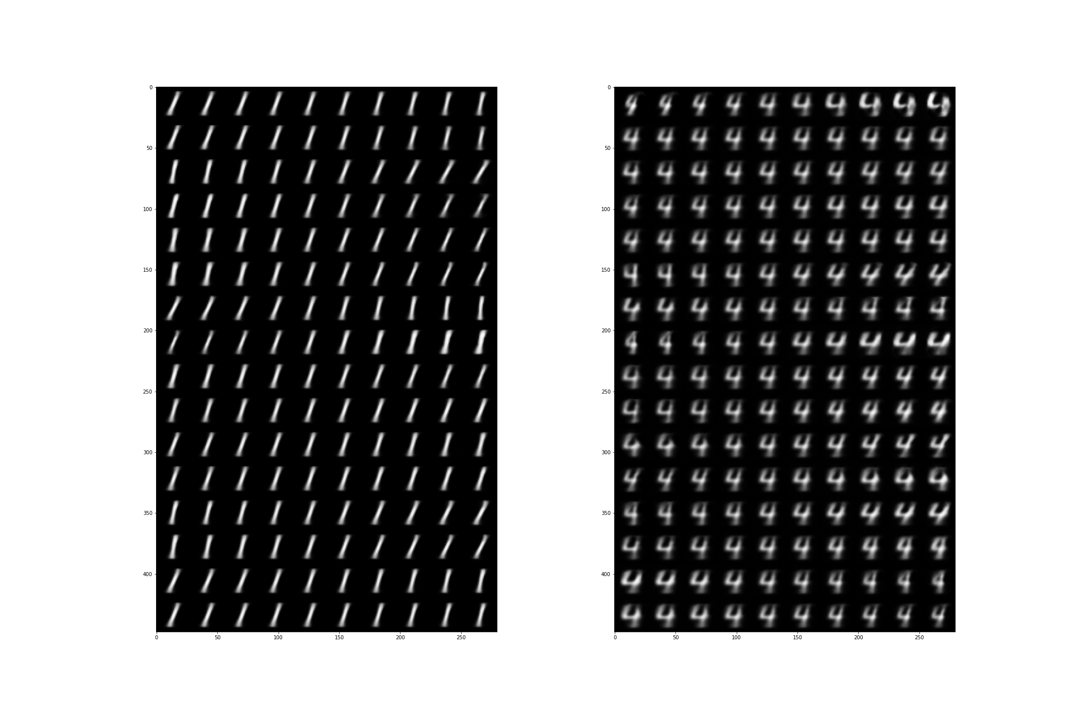
下面的代码调整每个功能，并在[-0.25，0.25]范围内以0.05的增量进行调整。 在每个点上，都会生成图像并将其存储在数组中。 因此，我们可以看到每个特征如何促进图像重建。

col = np.zeros((28,308))
for i in range(16): 
    feature_ = temp_features.copy()
    feature_[:,:,index, i] += -0.25
    row = np.zeros((28,28))
    for j in range(10):
        feature_[:,:,index, i] += 0.05
        row = np.hstack([row, tf.reshape(model.regenerate_image(tf.convert_to_tensor(feature_)), (28,28)).numpy()])
    col = np.vstack([col, row])
    
plt.figure(figsize=(30,20))
plt.imshow(col[28:, 28:], cmap='gray')

See some samples of reconstruction in the image below. As we can see, some of the features control the brightness, angle of rotation, thickness, skew, etc.

请参见下图的一些重建示例。 我们可以看到，某些功能控制着亮度，旋转角度，厚度，偏斜度等。

Reconstruction of Images by tweaking the features (Image by author)

通过调整功能重建图像(作者提供的图像)

结论 (Conclusion)

In this article, we have tried to reproduce the results as well as visualize the features described in the paper. The training accuracy is 99% and the testing accuracy is almost 98% which is really great. Although, the model takes a lot of time to train, but the features are very intuitive.

在本文中，我们试图重现结果并可视化本文中描述的功能。 训练精度为99％，测试精度几乎为98％，这确实很棒。 虽然，该模型需要花费很多时间进行训练，但是功能非常直观。

Github Repository: https://github.com/dedhiaparth98/capsule-network

Github存储库： https : //github.com/dedhiaparth98/capsule-network

翻译自: https://towardsdatascience.com/implementing-capsule-network-in-tensorflow-11e4cca5ecae

在流中抛出张量