


cc和毫升换算
As pointed out in Part 1 where we covered the concept of Association Analysis, analytics is increasingly becoming more augmented and relational. As a digital analyst, it's better for us to be aware of the connection between different data sources and be ready to produce much more than just descriptive analytics.
正如在第1部分中介绍了关联分析的概念所指出的那样,分析越来越变得越来越增强和关联。 作为数字分析师,让我们意识到不同数据源之间的联系,并准备进行更多的工作,不仅仅是描述性分析,还是更好的选择。
With this necessity in mind, we will cover another smart digital analytics concept — Customer Lifetime Value.
考虑到这一必要性,我们将介绍另一个智能数字分析概念-客户生命周期价值。
计算寿命值 (Calculating Lifetime Value)
Customer lifetime value (CLV) is the discounted sum of future cash flows attributed to the relationship with a customer. CLV estimates the ‘profit’ that an organization will derive from a customer in the future. The CLV can be used to evaluate the amount of money that can reasonably be devoted to customer acquisition. Even without considering the dollar value, CLV modeling still helps in identifying the most important (aka. profitable) customer segments which can then receive different treatment in terms of the acquisition strategy.
客户生命周期价值(CLV)是归因于与客户关系的未来现金流量的折现总和。 CLV估计组织将来将从客户中获得的“利润”。 CLV可用于评估可合理用于客户获取的金额。 即使不考虑美元价值,CLV建模仍然可以帮助确定最重要的(又称为获利的)客户群,这些客户群随后可以根据收购策略获得不同的待遇。
The taxonomy of CLV models depends much on the nature of the business. If the business has a contractual relationship (eg. subscription model) with customers then the most important issue in these situations is retaining customers over time, and survival analysis models are used to study the time until a customer cancels. These models are sometimes also referred to as ‘gone for good’ models because the models assume customers who cancel the service will not return.
CLV模型的分类法在很大程度上取决于业务的性质。 如果企业与客户之间有合同关系(例如,订阅模型),则在这种情况下,最重要的问题是随着时间的推移保留客户,而生存分析模型则用于研究直到客户取消之前的时间。 这些模型有时也称为“为善”,因为这些模型假定取消服务的客户不会再回来。
A simplistic CLV formula for a typical ‘gone for good’ models -
对于典型的“一劳永逸”模型,一种简单的CLV公式-
The CLV formula multiplies the per-period cash margin, $M, by a long-term multiplier that represents the present value of the customer relationship’s expected length:
CLV公式将每个期间的现金保证金$ M乘以一个长期乘数,该乘数代表客户关系的预期长度的现值:
CLV = $M [r / 1 + d-r]
CLV = $ M [r / 1 + dr]
where r is the per-period retention rate and d is the per-period discount rate.
其中r是每个时期的保留率, d是每个时期的折现率。
The other main class of CLV models is called ‘always a share.’ These models do not assume that customer inactivity implies the customer will never return. For example, a retail customer who does not buy this month might come back next month.
CLV模型的另一个主要类别称为“总是共享”。 这些模型不假定客户不活动意味着客户永远不会回来。 例如,本月不购买的零售客户可能在下个月回来。
It is these types of CLV models that are most relevant for an online retail business setup where users engage with the business at will, such as in e-commerce stores in which users might make purchases at any time.
这些类型的CLV模型与在线零售业务设置最相关,在在线零售业务设置中,用户可以随意从事业务,例如在电子商务商店中,用户可以随时进行购买。
In this article, I elaborate on one of the models that can be utilized to predict future CLV based on the customer’s historical transactions with the business. The model that is described in this series is best applied to predict the future value for existing customers who have at least a moderate amount of transaction history.
在本文中,我详细介绍了可用于基于客户与企业的历史交易来预测未来CLV的模型之一。 本系列中描述的模型最适用于预测至少具有中等交易历史记录的现有客户的未来价值。
购买CLV的概率模型 (Buy Till you Die Probabilistic models for CLV)
The BTYD models capture the non-contractual purchasing behavior of customers — or, more simply, models that tell the story of people buying until they die (become inactive as customers).
BTYD模型捕获了客户的非合同购买行为,或者更简单地说,是一个描述人们购买直到死亡的模型(成为不活跃的客户)。
There are 2 models widely used -
有2种广泛使用的模型-
Pareto/NBD
帕累托/ NBD
BG/NBD
BG / NBD
The BG/NBD (Beta Geometric Negative Binomial Distribution) model is easier to implement than Pareto/NBD and runs faster (I am intentionally being naive). The two models tend to yield similar results. These models assume probabilistic distribution of rates at which customers make purchases and the rate at which they drop out. The modeling is based on four parameters that describe these assumptions.
BG / NBD(贝塔几何负二项分布)模型比Pareto / NBD更易于实现,并且运行速度更快(我故意天真)。 这两个模型往往会产生相似的结果。 这些模型假设客户进行购买的速率和他们退出的速率的概率分布。 建模基于描述这些假设的四个参数。
Statistical introduction to the assumptions is important but out of the scope of this article. A high-level idea to keep in mind is that these models assume that the interactions of the customers with your business should be at their own will (in other words, random for your interpretation). If you have any influence (campaigns or promotional offers) in acquiring your customers, then that sort of historical data is not ideal to fit in these models.
对假设进行统计介绍很重要,但不在本文讨论范围之内。 要记住的一个高级想法是,这些模型假定客户与您的业务之间的交互应该是他们自己的意愿(换句话说,对于您的解释是随机的)。 如果您在吸引客户方面有任何影响力(活动或促销优惠),那么这种历史数据就不适合这些模型。
示例实施 (Example Implementation)
Let's consider the following scenario -
让我们考虑以下情况-
A retailer is re-strategizing their CPC ads. They want to understand who their most profitable customers are and what is the demography of this ideal customer. Eventually, they want to better target their CPC ads to get the most profitable customers possible. They have provided you with the last couple of years of transaction data and expect and output in terms of three customer buckets — high, medium, and low value. They expect to feed this customer value identifier back to their data lake and understand more about associated demographies for each bucket.
零售商正在重新制定其每次点击费用广告的策略。 他们想了解最赚钱的客户是谁,以及这个理想客户的人口统计是什么。 最终,他们希望更好地定位每次点击费用广告,以吸引尽可能多的获利客户。 他们为您提供了最近几年的交易数据,并根据三个客户群(高,中和低价值)期望和输出。 他们希望将这个客户价值标识符反馈给他们的数据湖,并了解有关每个存储桶的相关人口统计的更多信息。
We apply the model on a public dataset (details in citation). The dataset has transactions for the year 2010–11. We will first be preparing the data to shape it in the expected ‘event log’ format for the model. An event log is basically a log of each customer’s purchase with a record of revenue and timestamp associated with it. We will then be using a probabilistic model to calculate CLV. The data is enough to extract Recency, Frequency, and Monetary (RFM) values. The solution here uses an existing BTYD library in R.
我们将模型应用于公共数据集(详细引用)。 该数据集具有2010-11年的交易记录。 我们将首先准备数据以使其以模型的预期“事件日志”格式成形。 事件日志基本上是每个客户的购买日志,并带有与之相关的收入和时间戳记录。 然后,我们将使用概率模型来计算CLV。 该数据足以提取新近度,频率和货币(RFM)值。 这里的解决方案使用R中现有的BTYD库。
Please refer my GitHub for complete code -
请参考我的GitHub获取完整代码-
###########################################################################
#
# CLV Analysis: BG/ NBD Probabilistic Model
#
#
# Script:
# Generting clv predictions from retail transaction dataset
#
#
# Abhinav Sharma
###########################################################################


# Loading required libraries
library(lubridate)
library(BTYD)
library(BTYDplus)
library(dplyr)
library(ggplot2)


# reading the transaction dataset
df <- read.csv("Online Retail.csv", header = TRUE)
head(df)


range(df$InvoiceDate)


# We would need an additional column for Sales which will be Quantity times UnitPrice
df <- mutate(df, Sales = df$Quantity*df$UnitPrice)
head(df)


# keep only records with customer ID
colSums(is.na(df))
df <- na.omit(df)


# keeping only required columns
elog = df %>% group_by(CustomerID,InvoiceDate) %>% summarise(Sales = sum(Sales))
elog <- as_tibble(elog)
head(elog)


# Removing zero sales (purchase and returns on same date)
elog <- dplyr::filter(elog, elog$Sales!=0)
head(elog)


#  we convert the dates in the event log to R Date objects and rename the columns for use in helper functions
elog$InvoiceDate <- as.character(elog$InvoiceDate)
elog$InvoiceDate <- as.Date(elog$InvoiceDate, "%Y%m%d")
names(elog)[1] <- "cust"
names(elog)[2] <- "date"
names(elog)[3] <- "sales"
elog$cust <- as.factor(elog$cust)
str(elog)


# Weekly transaction Analysis
op <- par(mfrow = c(1, 2), mar = c(2.5, 2.5, 2.5, 2.5))
# incremental
weekly_inc_total <- elog2inc(elog, by = 7, first = TRUE)
weekly_inc_repeat <- elog2inc(elog, by = 7, first = FALSE)
plot(weekly_inc_total, typ = "l", frame = FALSE, main = "Incremental")
lines(weekly_inc_repeat, col = "red")
# commualtive
weekly_cum_total <- elog2cum(elog, by = 7, first = TRUE)
weekly_cum_repeat <- elog2cum(elog, by = 7, first = FALSE)
plot(weekly_cum_total, typ = "l", frame = FALSE, main = "Cumulative")
lines(weekly_cum_repeat, col = "red")
par(op)


# Convert Transaction logs to CBS format
calibration_cbs = elog2cbs(elog, units = "week", T.cal = "2011-10-01")
head(calibration_cbs)


# estimate parameters for the model
params.bgnbd <- BTYD::bgnbd.EstimateParameters(calibration_cbs) # BG/NBD
row <- function(params, LL) {
  names(params) <- c("k", "r", "alpha", "a", "b")
  c(round(params, 3), LL = round(LL))
}
rbind(`BG/NBD` = row(c(1, params.bgnbd),
                     BTYD::bgnbd.cbs.LL(params.bgnbd, calibration_cbs)))


# aggregate level dynamics can be visualized with the help of mbgcnbd.PlotTrackingInc
nil <- bgnbd.PlotTrackingInc(params.bgnbd,
                             T.cal = calibration_cbs$T.cal,
                             T.tot = max(calibration_cbs$T.cal + calibration_cbs$T.star),
                             actual.inc.tracking = elog2inc(elog))


# mean absolute error (MAE)
mae <- function(act, est) {
  stopifnot(length(act)==length(est))
  sum(abs(act-est)) / sum(act)
}
mae.bgnbd <- mae(calibration_cbs$x.star, calibration_cbs$xstar.bgnbd)
rbind(
  `BG/NBD` = c(`MAE` = round(mae.bgnbd, 3)))


# Parameters for gamma spend
spend_df = elog %>%
  group_by(cust) %>%
  summarise(average_spend = mean(sales),
            total_transactions = n())
spend_df$average_spend <- as.integer(spend_df$average_spend)
spend_df <- filter(spend_df, spend_df$average_spend>0)


head(spend_df)


# parameter values for our Gamma-Gamma spend model
gg_params = spend.EstimateParameters(spend_df$average_spend,
                                     spend_df$total_transactions)
gg_params


# Applying model to entire cohort
customer_cbs = elog2cbs(elog, units = "week")
customer_expected_trans <- data.frame(cust = customer_cbs$cust,
                                      expected_transactions =
                                        bgnbd.ConditionalExpectedTransactions(params = params.bgnbd,
                                                                              T.star = 12,
                                                                              x = customer_cbs[,'x'],
                                                                              t.x = customer_cbs[,'t.x'],
                                                                              T.cal  = customer_cbs[,'T.cal']))
customer_spend = elog %>%
  group_by(cust) %>%
  summarise(average_spend = mean(sales),
            total_transactions = n())
customer_spend <- filter(customer_spend, customer_spend$average_spend>0)
customer_expected_spend = data.frame(cust = customer_spend$cust,
                                     average_expected_spend =
                                       spend.expected.value(gg_params,
                                                            m.x = customer_spend$average_spend,
                                                            x = customer_spend$total_transactions))


# Combining these two data frames together gives us the next quarter customer value for each person in our data set.
merged_customer_data = customer_expected_trans %>%
  full_join(customer_expected_spend) %>%
  mutate(clv = expected_transactions * average_expected_spend,
         clv_bin = case_when(clv >= quantile(clv, .9, na.rm = TRUE) ~ "high",
                             clv >= quantile(clv, .5, na.rm = TRUE) ~ "medium",
                             TRUE ~ "low"))
head(merged_customer_data)
merged_customer_data %>%
  group_by(clv_bin) %>%
  summarise(n = n())


# Combining historical spend and forecast togather and saving it as an output csv
customer_clv <- left_join(spend_df, merged_customer_data, by ="cust")
head(customer_clv)
write.csv(customer_clv, "clv_output.csv")


# Plot of CLV Clusters
customer_clv  %>%
  ggplot(aes(x = total_transactions,
             y = average_spend,
             col = as.factor(clv_bin),
             shape = clv_bin))+
  geom_point(size = 4,alpha = 0.5)
Leaving out the upload and data cleaning part (where we convert the dataset into event log format), here is the breakdown of the remaining code —
省略了上传和数据清理部分(将数据集转换为事件日志格式),剩下的代码细分如下:
每周交易分析 (Weekly transaction Analysis)
Methods elog2cum and elog2inc take an event log as a first argument and count for each time unit the cumulated or incremental number of transactions. If the argument first is set to TRUE, then a customer’s initial transaction will be included, otherwise not.
方法elog2cum和elog2inc将事件日志作为第一个参数,并针对每个时间单位对事务的累积或增量计数。 如果将参数first设置为TRUE,则将包括客户的初始交易,否则不包括。
op <- par(mfrow = c(1, 2), mar = c(2.5, 2.5, 2.5, 2.5))
# incremental
weekly_inc_total <- elog2inc(elog, by = 7, first = TRUE)
weekly_inc_repeat <- elog2inc(elog, by = 7, first = FALSE)
plot(weekly_inc_total, typ = "l", frame = FALSE, main = "Incremental")
lines(weekly_inc_repeat, col = "red")
# commualtive
weekly_cum_total <- elog2cum(elog, by = 7, first = TRUE)
weekly_cum_repeat <- elog2cum(elog, by = 7, first = FALSE)
plot(weekly_cum_total, typ = "l", frame = FALSE, main = "Cumulative")
lines(weekly_cum_repeat, col = "red")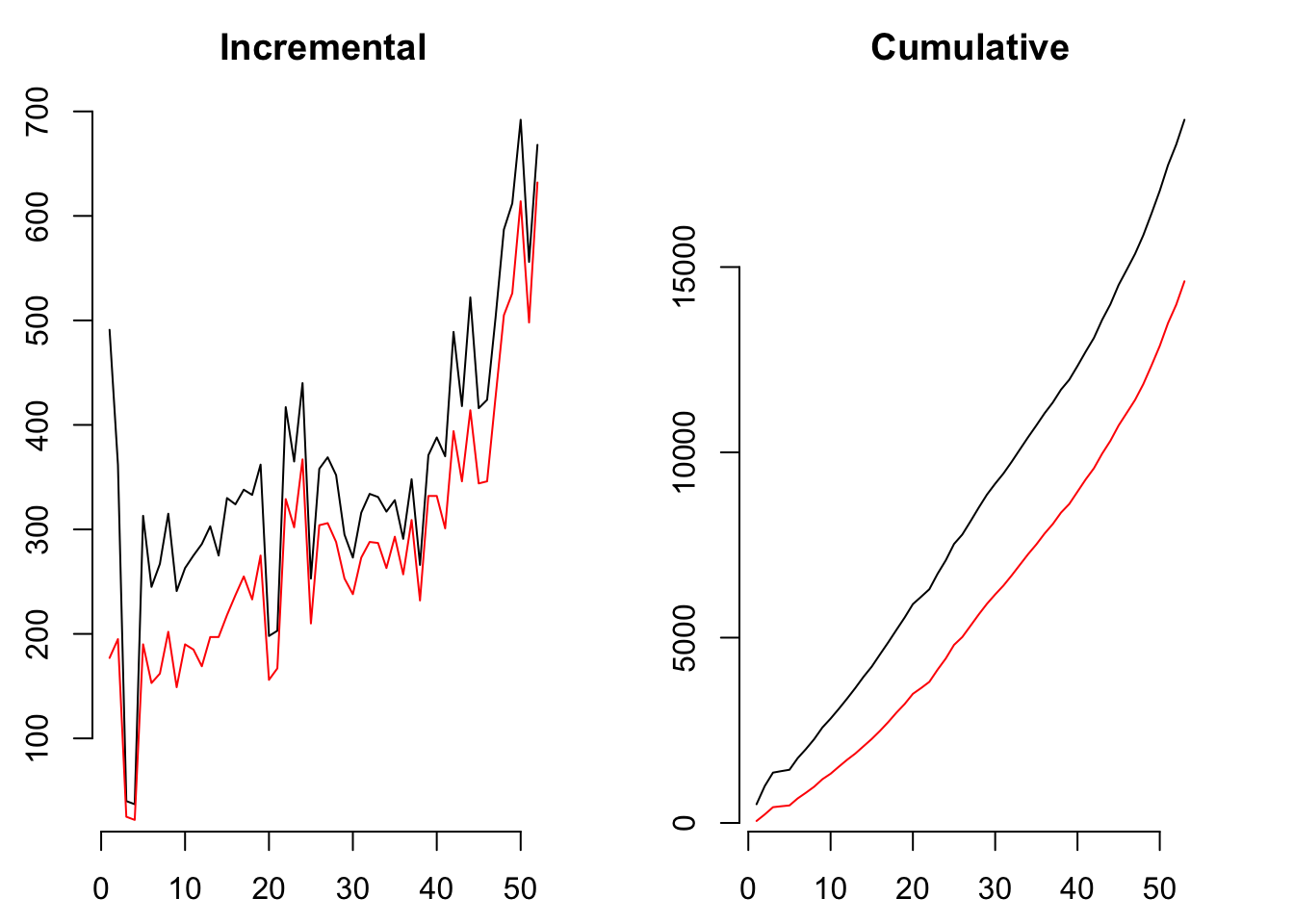
Further, we need to convert the event log into a customer-by-sufficient-statistic (CBS) format. The elog2cbs method is an efficient implementation for the conversion of an event log into CBS data.frame, with a row for each customer. This is the required data format for estimating model parameters. Argument T.cal allows one to calculate the summary statistics for a calibration and a holdout period separately.
此外,我们需要将事件日志转换为按客户统计的(CBS)格式。 elog2cbs方法是将事件日志转换为CBS data.frame的有效实现,每个客户都有一行。 这是估计模型参数所需的数据格式。 参数T.cal允许人们分别计算校准和保持期的汇总统计信息。
Instead of realistic calibration and holdout, I would like to use T.cal to sample only transactions before the holiday shopping for 2011, where there is an incremental spike. This will keep the estimated parameters realistic for future predictions.
我希望使用T.cal来代替2011年假期购物之前的交易,而不是进行实际的校准和保留,因为这里会有一个增量的峰值。 这将使估计的参数对于未来的预测保持现实。
calibration_cbs = elog2cbs(elog, units = "week", T.cal = "2011-10-01")
head(calibration_cbs)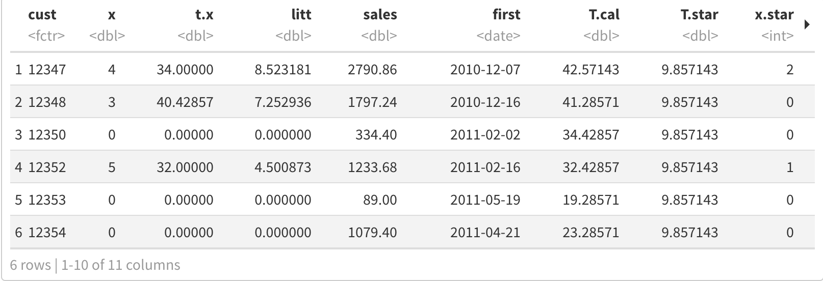
The returned field cust is the unique customer identifier, x the number of repeat transactions (i.e., frequency), t.x the time of the last recorded transaction (i.e., recency), litt the sum over logarithmic intertransaction times (required for estimating regularity), first the date of the first transaction, and T.cal the duration between the first transaction and the end of the calibration period. The time unit for expressing t.x, T.cal and litt are determined via the argument units, which is passed forward to method difftime, and defaults to weeks. Only those customers are contained, who have had at least one event during the calibration period.
返回的字段客户是唯一的客户标识符,x重复交易的数量(即频率),tx上次记录的交易的时间(即新近度),是对数交互时间的总和(用于估计规律性),首先是第一笔交易的日期,然后T.cal在第一笔交易和校准周期结束之间的持续时间。 表示tx,T.cal和litt的时间单位是通过参数单位确定的,该时间单位将传递给difftime方法,默认为周。 仅包含那些在校准期间至少发生过一次事件的客户。
- cust: Customer id (unique key). 客户:客户ID(唯一键)。
- x: Number of recurring events in calibration period. x:在校准期间内重复发生的事件数。
- t.x: Time between first and last event in calibration period. tx:校准周期中第一个事件和最后一个事件之间的时间。
- litt: Sum of logarithmic intertransaction timings during calibration period. 升:校准期间对数交互交易时间的总和。
- sales: Sum of sales in calibration period, incl. initial transaction. 销售:校准期内的销售总和,包括初始交易。
- first: Date of first transaction in calibration period. first:校准期内首次交易的日期。
- T.cal: Time between first event and end of calibration period. T.cal:第一次事件到校准周期结束之间的时间。
- T.star: Length of holdout period. T.star:保留期的长度。
- x.star: Number of events within holdout period. x.star:保持时间内的事件数。
- sales.star: Sum of sales within holdout period. sales.star:保留期内的销售总和。
Estimating the parameter values of the BG/NBD process.
估计BG / NBD过程的参数值。
# estimate parameters for various models
params.bgnbd <- BTYD::bgnbd.EstimateParameters(calibration_cbs) # BG/NBD
row <- function(params, LL) {
names(params) <- c("k", "r", "alpha", "a", "b")
c(round(params, 3), LL = round(LL))
}
rbind(`BG/NBD` = row(c(1, params.bgnbd),
BTYD::bgnbd.cbs.LL(params.bgnbd, calibration_cbs)))##        k     r alpha     a     b     LL
## BG/NBD 1 0.775 7.661 0.035 0.598 -29637
预测保留期 (Predicting on holdout period)
# predicting on holdout
calibration_cbs$xstar.bgnbd <- bgnbd.ConditionalExpectedTransactions(
params = params.bgnbd, T.star = 9,
x = calibration_cbs$x, t.x = calibration_cbs$t.x,
T.cal = calibration_cbs$T.cal)
# compare predictions with actuals at aggregated level
rbind(`Actuals` = c(`Holdout` = sum(calibration_cbs$x.star)),
`BG/NBD` = c(`Holdout` = round(sum(calibration_cbs$xstar.bgnbd))))##         Holdout
## Actuals    4308
## BG/NBD     2995
Comparing the predictions at an aggregate level, we see that the BG/NBD ‘under predicts’ for the dataset. That is attributed to the high jump in transactions during the holdout period (Nov and Dec 2011). The aggregate level dynamics can be visualized with the help of bgcnbd.PlotTrackingInc
在总体水平上比较预测,我们看到数据集的BG / NBD处于“预测不足”状态。 这是由于在保留期内(2011年11月和2011年12月),交易量激增。 可以通过bgcnbd.PlotTrackingInc可视化聚合级别的动态
nil <- bgnbd.PlotTrackingInc(params.bgnbd,
T.cal = calibration_cbs$T.cal,
T.tot = max(calibration_cbs$T.cal + calibration_cbs$T.star),
actual.inc.tracking = elog2inc(elog))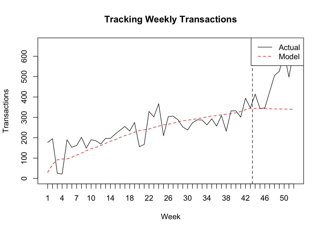
In case testing the model, we can use the holdout period to calculate MAE
在测试模型的情况下,我们可以使用保留期来计算MAE
# mean absolute error (MAE)
mae <- function(act, est) {
stopifnot(length(act)==length(est))
sum(abs(act-est)) / sum(act)
}
mae.bgnbd <- mae(calibration_cbs$x.star, calibration_cbs$xstar.bgnbd)
rbind(
`BG/NBD` = c(`MAE` = round(mae.bgnbd, 3)))##          MAE
## BG/NBD 0.769
伽玛支出参数 (Parameters for gamma spend)
Now we need to develop a model for the average transaction value for a customer. We will use a two-layered hierarchical model. The average transaction value will be Gamma distributed with shape parameter p. The scale parameter of this Gamma distribution is also Gamma distributed, with shape and scale parameters q and $$, respectively. Estimating these parameters requires the data to be in a slightly different format than the cbs format we used for the BG/NBD model. Instead, we simply need the average transaction value and the total number of transactions for each customer. This is easily obtained using dplyr notation on the elog object.
现在我们需要为客户的平均交易价值开发一个模型。 我们将使用两层的层次模型。 平均交易价值将为Gamma分布,形状参数为p 。 此Gamma分布的比例参数也是Gamma分布,其形状和比例参数分别为q和$$。 估算这些参数要求数据的格式与我们用于BG / NBD模型的cbs格式略有不同。 相反,我们仅需要每个客户的平均交易价值和交易总数。 使用elog对象上的dplyr表示法可以轻松实现这一点。
spend_df = elog %>%
    group_by(cust) %>%
    summarise(average_spend = mean(sales),
              total_transactions = n())## `summarise()` ungrouping output (override with `.groups` argument)spend_df$average_spend <- as.integer(spend_df$average_spend)
spend_df <- filter(spend_df, spend_df$average_spend>0)

  head(spend_df)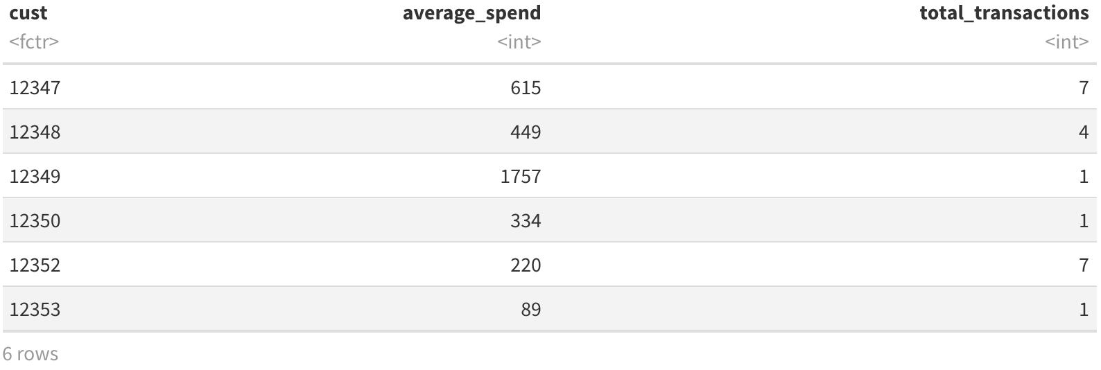
Now let’s plug this formatted data into the spend.EstimateParameters() function from the BTYD package to get the parameter values for our Gamma-Gamma spend model.
现在,让我们将这种格式化的数据插入BTYD包中的throw.EstimateParameters()函数中,以获取Gamma-Gamma支出模型的参数值。
gg_params = spend.EstimateParameters(spend_df$average_spend,
                                       spend_df$total_transactions)
  gg_params## [1]   2.619805   3.346577 313.666656
将模型应用于整个队列 (Applying the model to the entire cohort)
With all the parameters needed to understand the transaction and average revenue behavior, we can now apply this model to our entire cohort of customers. To do so, we will need to create a cbs data frame for our entire data set (i.e., no calibration period). We can make use of the elog2cbs() function again, but omit the calibration_date argument. We can then calculate expected transactions and average transaction value for the next 12 weeks for each customer.
有了了解交易和平均收入行为所需的所有参数,我们现在可以将此模型应用于整个客户群。 为此,我们将需要为整个数据集创建一个cbs数据帧(即没有校准周期)。 我们可以再次使用elog2cbs()函数,但是忽略了Calibration_date参数。 然后,我们可以计算每个客户未来12周的预期交易和平均交易价值。
customer_cbs = elog2cbs(elog, units = "week")
customer_expected_trans <- data.frame(cust = customer_cbs$cust,
                                      expected_transactions =
                                        bgnbd.ConditionalExpectedTransactions(params = params.bgnbd,
                                                                              T.star = 12,
                                                                              x = customer_cbs[,'x'],
                                                                              t.x = customer_cbs[,'t.x'],
                                                                              T.cal  = customer_cbs[,'T.cal']))
customer_spend = elog %>%
  group_by(cust) %>%
  summarise(average_spend = mean(sales),
            total_transactions = n())## `summarise()` ungrouping output (override with `.groups` argument)customer_spend <- filter(customer_spend, customer_spend$average_spend>0)
customer_expected_spend = data.frame(cust = customer_spend$cust,
                                     average_expected_spend =
                                        spend.expected.value(gg_params,
                                                             m.x = customer_spend$average_spend,
                                                             x = customer_spend$total_transactions))
Combining these two data frames together gives us the next three month’s worth of customer value for each person in our data set. We can further bucket them into high, medium, and low categories.
将这两个数据框组合在一起,可以为我们数据集中的每个人提供接下来三个月的客户价值。 我们可以进一步将它们分为高,中和低类别。
merged_customer_data = customer_expected_trans %>%
  full_join(customer_expected_spend) %>%
  mutate(clv = expected_transactions * average_expected_spend,
         clv_bin = case_when(clv >= quantile(clv, .9, na.rm = TRUE) ~ "high",
                             clv >= quantile(clv, .5, na.rm = TRUE) ~ "medium",
                             TRUE ~ "low"))merged_customer_data %>%
  group_by(clv_bin) %>%
  summarise(n = n())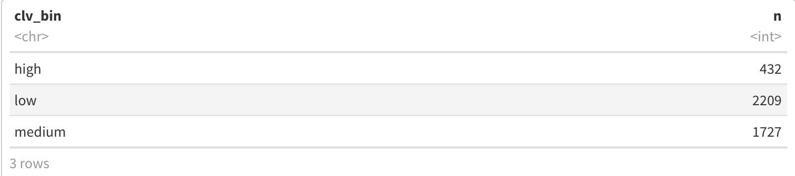
Combining historical spend and forecast together and saving it as an output csv —
将历史支出和预测结合在一起,并将其保存为输出csv,
customer_clv <- left_join(spend_df, merged_customer_data, by ="cust")
head(customer_clv)
write.csv(customer_clv, "clv_output.csv")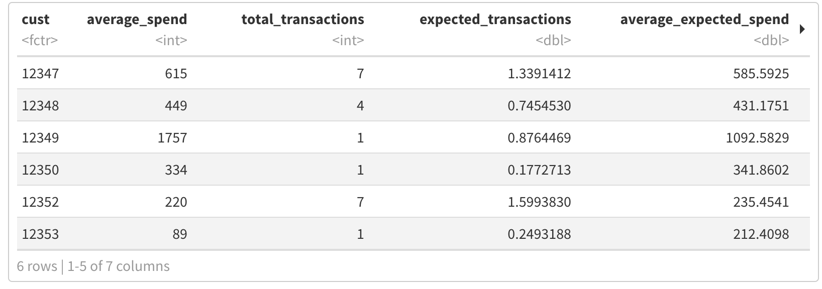
CLV群集图(Plot of CLV Clusters)
customer_clv  %>%
    ggplot(aes(x = total_transactions,
               y = average_spend,
               col = as.factor(clv_bin),
               shape = clv_bin))+
    geom_point(size = 4,alpha = 0.5)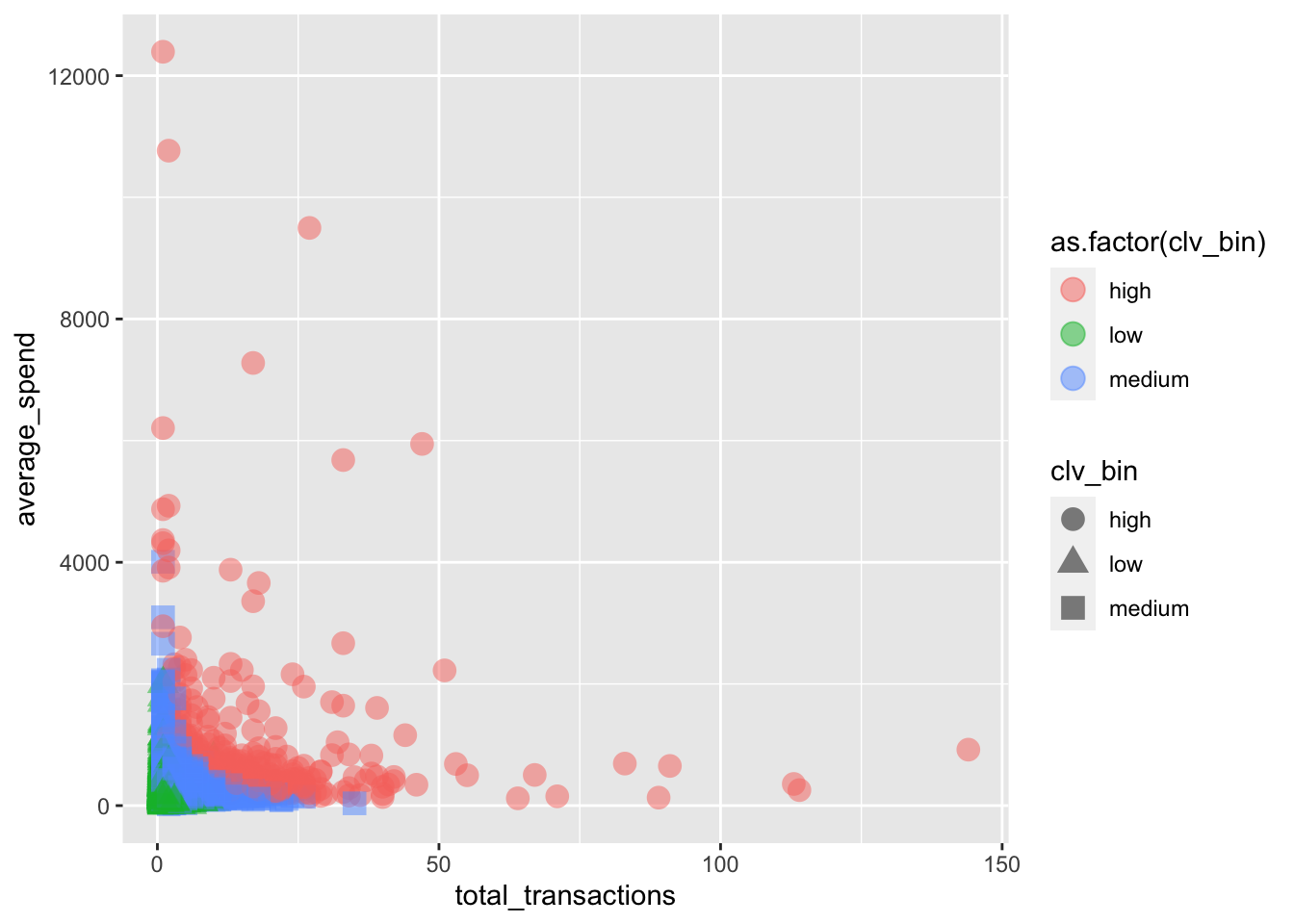
The output csv can now be fed back to and merged with the customer database. The clv bucket metric will then be available for breaking down in terms of other demographic or behavioral information.
现在可以将输出csv反馈到客户数据库并与客户数据库合并。 然后,就可以根据其他人口统计或行为信息细分clv bucket指标。
引文 (Citation)
Daqing Chen, Sai Liang Sain, and Kun Guo, Data mining for the online retail industry: A case study of RFM model-based customer segmentation using data mining, Journal of Database Marketing and Customer Strategy Management, Vol. 19, №3, pp. 197–208, 2012 (Published online before print: 27 August 2012. doi: 10.1057/dbm.2012.17).
Daqing Chen,Sai Liang Sain和Kun Kun,在线零售行业的数据挖掘:使用数据挖掘的基于RFM模型的客户细分的案例研究,《数据库营销与客户战略管理》,第1卷。 19,№3,第197–208页,2012年(印刷前在线发布:2012年8月27日。doi:10.1057 / dbm.2012.17)。
cc和毫升换算


 1万+
1万+

 被折叠的 条评论
为什么被折叠?
被折叠的 条评论
为什么被折叠?
 到【灌水乐园】发言


