


 本文深入研究了dask数据框在大数据处理中的使用,详细解析了dask如何提供并行计算能力以高效处理大规模数据。通过对dask框架的理解,读者可以提升在python环境中进行大数据分析的能力。
dask 大数据
Pandas, but for big data
熊猫,但大数据
Ever dealt with dataframes several GBs in size, perhaps exceeding the capacity of the RAM in your local machine? Pandas can’t handle dataframes larger than your RAM. Trust me, I’ve tried it. I clearly remember the aftermath: the background song playing in YouTube interrupted intermittently and then stopped altogether, my machine hung up, and finally, my screen turned black, all in quick succession. I also remember panicking at the thought of having inflicted some permanent damage on my laptop. Much to my relief, a power cycle brought my laptop back to life.
是否曾经处理过数GB的数据帧,也许超出了本地计算机中RAM的容量? 熊猫无法处理大于RAM的数据帧。 相信我,我已经尝试过了。 我清楚地记得后果:在YouTube中播放的背景歌曲断断续续地中断,然后完全停止,我的机器挂起,最后,我的屏幕变黑了,很快就全部消失了。 我还记得对笔记本电脑造成永久损坏的想法感到惊慌。 令我大为欣慰的是,电源循环使我的笔记本电脑恢复了活力。
But then, how was I supposed to process this large dataframe? Usher in dask!
但是,我应该如何处理这个大数据帧呢? 迎接黄昏!
In this post, we will, as the title suggests, dive deep into dask dataframes. It should be evident by now that dask performs some magic that pandas can’t. We will essentially look at that magic, the ‘how’ behind the ‘wow’. The table of contents, listed below, will give you a fair idea of what to expect from this post.
正如标题所示,在这篇文章中,我们将深入研究Dask数据框架。 到现在为止,应该很明显,达斯库斯执行了熊猫无法做到的某些魔术。 我们将本质上看一看魔术,即“哇”背后的“方式”。 下面列出的目录将使您对这篇文章有什么期待。
什么是快? (What is dask?)
In layperson terms, dask is one of the popular gateways to parallel computing in python. So if your machine has 4 cores, it can utilize all 4 of them simultaneously for computation. There are dask equivalents for many popular python libraries like numpy, pandas, scikit-learn, etc. In this post, we are interested in the pandas equivalent: dask dataframes.
用非专业人士的话来说,dask是python中并行计算的流行网关之一。 因此,如果您的计算机具有4个内核,则可以同时利用所有4个内核进行计算。 许多流行的python库(例如numpy,pandas,scikit-learn等)都有dask等效项。在本文中,我们对pandas等效项感兴趣:dask数据帧。
解决RAM限制 (Addressing the RAM limitations)
Parallel computing is all good. But how does dask address the storage problem? Well, it breaks down the huge dataframe into several smaller pandas dataframes. But the cumulative size of the smaller dataframes is still larger than the RAM. So how does breaking down into smaller dataframes solve the problem? Well, dask stores each of these smaller pandas dataframes on your local storage (HDD/ SSD), and brings in data from the individual dataframes into the RAM as and when required. A typical PC has a local storage capacity of several 100 GBs while the RAM capacity is restricted to just a couple of GBs. Thus, dask allows you to process data much larger than your RAM capacity.
并行计算都很好。 但是,如何轻松解决存储问题? 好吧,它将巨大的数据框分解为几个较小的熊猫数据框。 但是,较小数据帧的累积大小仍大于RAM。 那么分解为较小的数据帧如何解决该问题呢? 好吧,dask将这些较小的熊猫数据帧中的每一个存储在本地存储(HDD / SSD)上,并在需要时将各个数据帧中的数据导入RAM中。 典型的PC具有几百GB的本地存储容量,而RAM容量仅限制为几个GB。 因此,dask使您可以处理比RAM容量大得多的数据。
To give an example, say your dataframe contains a billion rows. Now if you want to add two columns to create a third column, pandas would first load that entire dataframe into the RAM and then try to perform the computation. Sadly, depending on the size of your RAM, it may overwhelm your system in the data loading stage itself. Dask will break down the dataframe into, say 100 chunks. It will then bring in 1 chunk into the RAM, perform the computation, and send it back to the disk. It will repeat this with the other 99 chunks. If you have 4 cores in your machine, and your RAM can handle data equal to the size of 4 chunks, all of them will work in parallel and the operation will be completed in 1/4th of the time. The best part: you need not worry about the number of cores involved or the capacity of your RAM. Dask will figure out everything in the background and not give you any burden.
举个例子,假设您的数据框包含十亿行。 现在,如果您想添加两列以创建第三列,熊猫将首先将整个数据帧加载到RAM中,然后尝试执行计算。 遗憾的是,根据RAM的大小,它可能会在数据加载阶段本身使系统不堪重负。 Dask会将数据帧分解为100个大块。 然后它将1个块放入RAM,执行计算,然后将其发送回磁盘。 它将与其他99个块重复此操作。 如果您的计算机中有4个内核,并且RAM可以处理等于4个块的大小的数据,则它们将全部并行工作,并且该操作将在1/4的时间内完成。 最好的部分:您不必担心所涉及的内核数或RAM的容量。 Dask会找出后台的所有内容,不会给您带来任何负担。
Sounds good? So let’s begin our dive.
听起来不错? 因此,让我们开始潜水吧。
达斯克数据框剖析 (Anatomy of the Dask Dataframe)
We will be using a CSV file containing more than 74 million location coordinates. The file measures about 2.5 GB in size. Depending on the capacity of the usable RAM in your machine, this may or may not overwhelm your system using pandas. I’ll be using a quad-core machine having 12 GB RAM. So pandas could have comfortably handled this dataframe on my machine. This will be useful when we benchmark pandas and dask in a later post and help us understand when to use dask and when to use pandas.
我们将使用包含超过7400万个位置坐标的CSV文件。 该文件的大小约为2.5 GB。 根据计算机中可用RAM的容量,这可能会或可能不会使使用熊猫的系统不知所措。 我将使用具有12 GB RAM的四核计算机。 因此,熊猫本可以轻松地在我的机器上处理此数据帧。 当我们在以后的文章中对熊猫和熊猫进行基准测试时,这将很有用,并有助于我们了解何时使用熊猫以及何时使用熊猫。
Let’s read the CSV:
让我们阅读CSV:
import dask.dataframe as dd
df_dd = dd.read_csv('data/lat_lon.csv')
If you try to visualize the dask dataframe, you will get something like this:
如果尝试可视化dask数据框,则会得到以下内容:
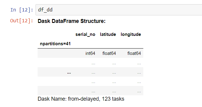
As you can see, unlike pandas, here we just get the structure of the dataframe and not the actual dataframe. If you think about it, it makes sense. Dask has loaded the dataframe in several chunks, which are present on the disk, and not in the RAM. If it has to output the dataframe, it will first need to bring all of them into the RAM, stitch them together and then showcase the final dataframe to you. It won’t do that until you force it to do so using .compute() . More on that later.
如您所见,与熊猫不同,这里我们仅获取数据框的结构,而不是实际数据框。 如果您考虑一下,这是有道理的。 Dask已将数据帧分为几块加载,这些块存在于磁盘上,而不存在于RAM中。 如果必须输出数据帧,则首先需要将所有数据帧都放入RAM,将它们缝合在一起,然后向您展示最终的数据帧。 除非您使用.compute()强迫它这样做,否则它不.compute() 。 以后再说。
The structure itself conveys a lot of information. For instance, it shows that the dataframe has been split into 41 chunks. It shows the columns in the dataframe and their data types. So far, so good. But hang on, what is the meaning of the last line, containing dask name and the number of tasks? What are these tasks? What is the significance of the name?
结构本身传达了很多信息。 例如,它表明数据帧已被分为41个块。 它显示了数据框中的列及其数据类型。 到目前为止,一切都很好。 但是,等等,最后一行的含义是什么,它包含任务名称和任务数? 这些任务是什么? 这个名字的意义是什么?
达斯克的任务图 (Dask’s Task Graph)
We can get a lot of these answers by invoking the .visualize() method. Let’s try it out. Please note that you will need the Graphviz library for this method to work.
通过调用.visualize()方法,我们可以获得很多这样的答案。 让我们尝试一下。 请注意,您将需要Graphviz库才能使用此方法。
df_dd.visualize()
Not quite legible, right? Let’s reduce the number of partitions and try. To reduce the number of partitions, we will read the CSV again, this time specifying a block size of 600MB.
不太清晰,对不对? 让我们减少分区数并尝试。 为了减少分区数量,我们将再次读取CSV,这一次指定600MB的块大小。
df_dd = dd.read_csv('data/lat_lon.csv',blocksize='600MB')Now, we can see that the dataframe has been broken down into 5 chunks.
现在,我们可以看到数据帧已分为5个块。

The df_dd.visualize() command’s output will now be more legible.
df_dd.visualize()命令的输出现在将更加清晰。
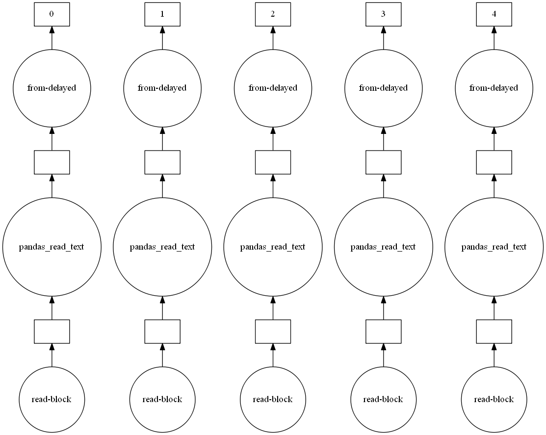
The above image represents a task graph in dask. Task graphs are dask’s way of representing parallel computations. The circles represent the tasks or functions and the squares represent the outputs/ results. As you can see, the process of creating the dask dataframe requires a total of 15 tasks, 3 tasks per partition. In general, the number of dask tasks will be a multiple of the number of partitions, unless we perform an aggregate computation, like max(). In the first step, it will read a block of 600 MB (it can be ≤ 600 MB for the last partition). It will then convert this block of bytes to a pandas dataframe in the next step. In the final step, it makes this dataframe ready for parallel computation using from_delayed.
上面的图像代表了一个任务图。 任务图是表示并行计算的dask方式。 圆圈代表任务或功能,正方形代表输出/结果。 如您所见,创建dask数据框的过程总共需要15个任务,每个分区3个任务。 通常,除非我们执行诸如max()类的聚合计算,否则轻快任务的数量将是分区数量的倍数。 在第一步中,它将读取一个600 MB的块(对于最后一个分区,它可以≤600 MB)。 然后,它将在下一步中将此字节块转换为pandas数据帧。 在最后一步中,它使用from_delayed使此数据帧准备好进行并行计算。
达斯克的懒惰 (Dask’s Laziness)
The delayed function lies at the core of parallelization in dask. As the name suggests, it delays the output of a computation, and instead, returns a lazy dask graph. You will see the word lazy repeat again and again in the official dask documentation. Why lazy? As per the official dask documentation, the dask graphs are lazy because:
delayed功能是dask并行化的核心。 顾名思义,它会延迟计算的输出,而是返回一个懒惰的dask图。 在正式的dask文档中,您会一次又一次地看到lazy一词。 为什么偷懒? 根据官方的dask文档 ,dask图是惰性的,因为:
Rather than compute their results immediately, they record what we want to compute as a task into a graph that we’ll run later on parallel hardware.
他们没有立即计算出结果,而是将要作为任务计算的结果记录在一个图形中,稍后将在并行硬件上运行。
Once dask has the entire task graph in front of it, it is much efficient to parallelize the computation.
一旦dask拥有了整个任务图,对计算进行并行化将非常有效。
Dask’s laziness will become more clear with the following example. Let us visualize the output of calling .max() on the dask dataframe.
通过以下示例,Dask的懒惰将变得更加清晰。 让我们可视化dask数据帧上调用.max()的输出。
df_dd.max().visualize()
As you can see, instead of computing the max value of each column, calling .max() just appended tasks to the original task graph. It added two steps. One is the computation of the max for each partition, and the other is the computation of the aggregate max.
如您所见,调用.max()而不是计算每列的最大值,只是将任务附加到原始任务图上。 它增加了两个步骤。 一个是每个分区的最大值的计算,另一个是聚合最大值的计算。
The lazy dask graph just mimics a lazy engineer. When given a problem, a competent but lazy engineer will just create the solution graph in his/her mind and let it stay there. Only when forced to provide the results (say by a deadline) will the engineer perform the computations. To get the results from the dask graph, we have to force it to perform the computations. We do that by calling the .compute() method.
懒惰的图形只是模仿了一个懒惰的工程师。 当遇到问题时,能干但懒惰的工程师只会在他/她的脑海中创建解决方案图,然后将其保留在那里。 只有当被迫提供结果(例如按期限)时,工程师才会执行计算。 为了从dask图获得结果,我们必须强制它执行计算。 我们通过调用.compute()方法来实现。
df_dd.max().compute()
>> serial_no    7.470911e+07
   latitude     1.657000e+02
   longitude    1.631770e+02
   dtype: float64
The CSV used has dummy data. So don’t worry about latitude being greater than 90 degrees.
所使用的CSV具有伪数据。 因此,不必担心纬度大于90度。
Before we go ahead, I’d just like to show you what would have happened had you chosen to invoke the repartition command instead of reading the CSV again with a specified block size.
在继续之前,我想向您展示如果您选择调用重新分区命令而不是再次读取具有指定块大小的CSV将会发生什么。
If we go back to the old dask dataframe with 41 partitions, and apply the repartition command and then run .visualize(), the output will be something like this:
如果我们回到具有41个分区的旧dask数据帧,并应用.visualize()命令,然后运行.visualize() ,则输出将如下所示:
df_dd = dd.read_csv('data/lat_lon.csv')
df_dd = df_dd.repartition(npartitions=5)
df_dd.visualize()
We have essentially increased the number of tasks. Repartitioning should be used only when you have reduced the original dataframe to a fraction of its size and no longer need a lot of partitions. To reduce the number of partitions right at the beginning, it is best to mention the blocksize while reading data.
我们实质上增加了任务数量。 仅当将原始数据帧减小到其大小的一小部分并且不再需要大量分区时,才应使用重新分区。 为了从一开始就减少分区数,最好在读取数据时提及块大小。
分区和索引 (Partitions and Indexing)
Let’s now look at the partitions of the dask dataframe. We can access the individual partitions with the .get_partition() method. Let’s call the first partition.
现在让我们看一下dask数据帧的分区。 我们可以使用.get_partition()方法访问各个分区。 我们称第一个分区。
df_0 = df_dd.get_partition(0)Let us look at the index range of this partition
让我们看一下该分区的索引范围
df_0.index.min().compute()
>> 0df_0.index.max().compute()
>> 17707567
Now, the rather surprising thing is that you will get approximately the same answer if you run these computations on the next partition.
现在,相当令人惊讶的是,如果在下一个分区上运行这些计算,您将得到大致相同的答案。
df_1 = df_dd.get_partition(1)
df_1.index.min().compute()
>> 0df_1.index.max().compute()
>> 17405554
What this means is that there is no common index spanning across the partitions. Each partition has its separate index. This can also be confirmed by accessing the dataframe divisions. The divisions contain the min value of each partition’s index and the max value of the last partition’s index.
这意味着没有跨分区的通用索引。 每个分区都有其单独的索引。 也可以通过访问数据帧分区来确认。 这些分区包含每个分区索引的最小值和最后一个分区索引的最大值。
df_dd.divisions
(None, None, None, None, None, None)
Here, since the partitions are independent and each has its separate index, dask doesn’t find a common index according to which the data is divided.
在这里,由于分区是独立的,并且每个分区都有其单独的索引,因此dask找不到用于划分数据的公共索引。
For a dataframe with no well-defined divisions, an operation like df_dd.loc[5:500] will make no sense. Each partition has indices from 5 to 500. If we have no column in the dataframe which can be used as an index, we simply can’t use index-based .loc.
对于没有明确定义的除法的数据帧,像df_dd.loc[5:500]类的操作将毫无意义。 每个分区的索引从5到500。如果我们在数据框中没有可以用作索引的列,则根本不能使用基于索引的.loc 。
Luckily, we have a serial number column which we can use as the index. We will have to inform the dask dataframe to use it as the index.
幸运的是,我们有一个序列号列,可以用作索引。 我们将必须通知dask数据框以将其用作索引。
df_dd = df_dd.set_index('serial_no')Please note that this is a costly operation, and shouldn’t be done again and again. It involves a lot of communication, shuffling, and exchange of data between the partitions. However, a one-time effort is worth it, if you need to perform frequent index-based slicing. After setting the index, if we check the divisions again, we will get the following output:
请注意,这是一项昂贵的操作,因此不应一次又一次地执行。 它涉及分区之间的大量通信,改组和数据交换。 但是,如果您需要执行频繁的基于索引的切片,那么一次性的工作是值得的。 设置索引后,如果再次检查除法,将得到以下输出:
df_dd.divisions
>> (0, 17707568, 35113123, 52512497, 69929691, 74709113)
Note that serial number will no longer be a separate column.
请注意,序列号将不再是单独的列。
df_dd.columns
>> Index(['latitude', 'longitude'], dtype='object')
Now, thanks to the indexing, each partition will have non-overlapping min and max indices.
现在,由于有了索引,每个分区将具有不重叠的最小和最大索引。
df_1 = df_dd.get_partition(1)
df_1.index.min().compute()
>> 17707568df_1.index.max().compute()
>> 35113122
Setting the index has some significant advantages if you need to slice by index. On the original dataframe, df_dd.loc[5:500].compute() takes about 42 seconds, and of course, the result is far from accurate, and the length of the result is n_partitions times the expected length. On the indexed dataframe, the same command takes just 4 seconds and returns the correct result.
如果需要按索引分片,则设置索引具有一些明显的优势。 在原始数据帧上, df_dd.loc[5:500].compute()大约需要42秒,当然,结果远非准确,结果的长度是n_partitions乘以预期长度。 在索引的数据帧上,同一命令仅需4秒钟,即可返回正确的结果。
下一步: (Next Steps:)
In this post, a pretty detailed examination of the dask dataframe was done. Now that you know how dask is different from pandas, you can move on to the next post, where we look at the parallelization of tasks using dask. While dask takes care of most of the parallelization itself, there are a few things you should know to fully take advantage of dask’s parallelization. See you in the next post (How to efficiently parallelize dask dataframe computations on a single machine), where we will discuss why calling .compute() may not be the most efficient way to calculate results.
在这篇文章中,对dask数据框进行了相当详细的检查。 现在您知道dask与pandas的区别是什么,您可以继续阅读下一篇文章 ,我们将在本文中探讨使用dask进行任务并行化。 虽然dask负责大部分并行化本身,但是您应该了解一些要充分利用dask并行化的知识。 在下一篇文章( 如何在一台机器上有效地并行化dask数据帧计算 )中见,我们将讨论为什么调用.compute()可能不是计算结果的最有效方法。
参考资料和有用资源: (References and Useful Resources:)
Dask is very well documented. You can have a look at the following resources to dive deeper into dask:
Dask有很好的记录。 您可以查看以下资源以更深入地研究:
Dask Documentation: https://docs.dask.org/en/latest/
达斯克文档: https ://docs.dask.org/en/latest/
Dask Tutorials: https://tutorial.dask.org/
达斯教程: https ://tutorial.dask.org/
Dask Tutorial Notebooks: https://github.com/dask/dask-tutorial
达斯教程笔记: https : //github.com/dask/dask-tutorial
Dask Examples: https://examples.dask.org/
Dask示例: https ://examples.dask.org/
翻译自: https://medium.com/@sanghviyash7/a-deep-dive-into-dask-dataframes-7455d66a5bc5
dask 大数据


 1671
1671

 被折叠的 条评论
为什么被折叠?
被折叠的 条评论
为什么被折叠?
 到【灌水乐园】发言


