python 量化策略回测_在python中创建和回测对交易策略

最新推荐文章于 2024-11-04 00:57:52 发布

weixin_26640581

最新推荐文章于 2024-11-04 00:57:52 发布

阅读量1.3k

点赞数

文章标签： python django

原文链接：https://medium.com/swlh/creating-and-back-testing-a-pairs-trading-strategy-in-python-caa807b70373

版权

本文介绍了如何在Python环境中创建并回测一对交易策略。通过详细的教程，读者将学习到如何利用Python进行量化交易策略的开发和验证。

摘要生成于 C知道，由 DeepSeek-R1 满血版支持，前往体验 >

python 量化策略回测

Pairs trading is one of the many mean-reversion strategies. It is considered non-directional and relative as it aims to trade on both related stocks with similar statistical and economical properties. It first identifies a historical relationship that has been recently broken and then buys the implied undervalued security while shorting the overvalued security in attempt to revert to the original relationship. We must first understand the difference between correlation and cointegration. Correlation (ρ) measures the degree of the linear relationship between variables, it has the following features:

货币对交易是许多均值回复策略之一。它被认为是无方向性和相对性的，因为它旨在买卖具有相似统计和经济特性的两种相关股票。它首先确定最近被破坏的历史关系，然后购买隐含的被低估的证券，同时卖空被高估的证券，以尝试恢复为原始关系。我们必须首先了解关联和协整之间的区别。相关度(ρ)度量变量之间的线性关系的程度，它具有以下特征：

ρ = -1, means a perfectly negative relationship. They move in the opposite direction.
ρ= -1，表示完全负关系。它们朝相反的方向移动。
ρ = 0, means there is no linear relationship between the two.
ρ= 0，表示两者之间没有线性关系。
ρ = 1, means a perfect linear relationship between the datasets. They move hand in hand.
ρ= 1，表示数据集之间的理想线性关系。他们携手并进。

Correlation does not imply causality. It is not used to explain variations in one dataset caused by the other. We use regression analysis for that issue. Negatively correlated assets can be used to hedge one another, and it is the basic diversification rule for portfolio management. If we have two different datasets and their two respective variances, we can calculate a measure called covariance. Covariance has the same principle as correlation except that it is unbounded and therefore not really meaningful. It is however used in the formula of correlation:

相关并不意味着因果关系。它不用于解释一个数据集由另一数据集引起的变化。对于该问题，我们使用回归分析。负相关的资产可以用来对冲，这是资产组合管理的基本多元化规则。如果我们有两个不同的数据集以及它们各自的两个方差，则可以计算一个称为协方差的度量。协方差与相关具有相同的原理，除了协方差是无界的，因此实际上没有意义。但是，它用在相关公式中：

If the correlation coefficient is zero, it does not necessarily mean that there is absolutely no relationship between the two datasets. It simply means that there is not a linear one.

如果相关系数为零，则不一定意味着两个数据集之间绝对没有关系。它仅表示没有线性关系。

Image for post — A chart showing perfect correlation between two datasets. Correlation = 1

Disclaimer: The below choice for the two related securities is inspired by Dr. Ernest Chan. The back-test to follow does not take into account the transaction costs and therefore the reality may differ with respect to the results found at the end of the article.

免责声明：两种相关证券的以下选择均受Ernest Chan博士的启发。遵循的回测未考虑交易成本，因此，对于本文结尾处的结果，实际情况可能有所不同。

We must be extremely cautious with correlation. With financial data you will most likely have to calculate correlations of returns and not prices. If you’re interested in short-term relationships, go for returns’ correlations, otherwise, opt for prices if you’re in it for the long-term. Cointegration, on the other hand, is not too dissimilar to correlation. In plain terms, it means that the ratio between the two financial time series will vary around a constant mean. Pairs trading can rely on the constant ratio that is expected to revert to its long-term mean (i.e. converge). Below are two ETFs with the following details:

我们对关联必须非常谨慎。使用财务数据，您最有可能必须计算收益而不是价格的相关性。如果您对短期关系感兴趣，请寻求收益的相关性，否则，如果您长期处于收益关系中，请选择价格。另一方面，协整与相关并不太相似。简而言之，这意味着两个财务时间序列之间的比率将围绕恒定的平均值变化。货币对交易可以依靠恒定比率，该比率有望恢复为长期均值(即收敛)。以下是两个具有以下详细信息的ETF：

EWA: iShares MSCI Australia ETF, seeks to replicate investment results that correspond to the price and yield performance of publicly traded securities in the Australian market.
EWA ：iShares MSCI澳大利亚ETF，力求复制与澳大利亚市场上公开交易证券的价格和收益表现相对应的投资结果。
EWC: iShares MSCI Canada ETF seeks to replicate investment results that correspond to the price and yield performance of publicly traded securities in the Canadian market.
EWC ：iShares MSCI加拿大ETF寻求复制与加拿大市场上公开交易证券的价格和收益表现相对应的投资结果。

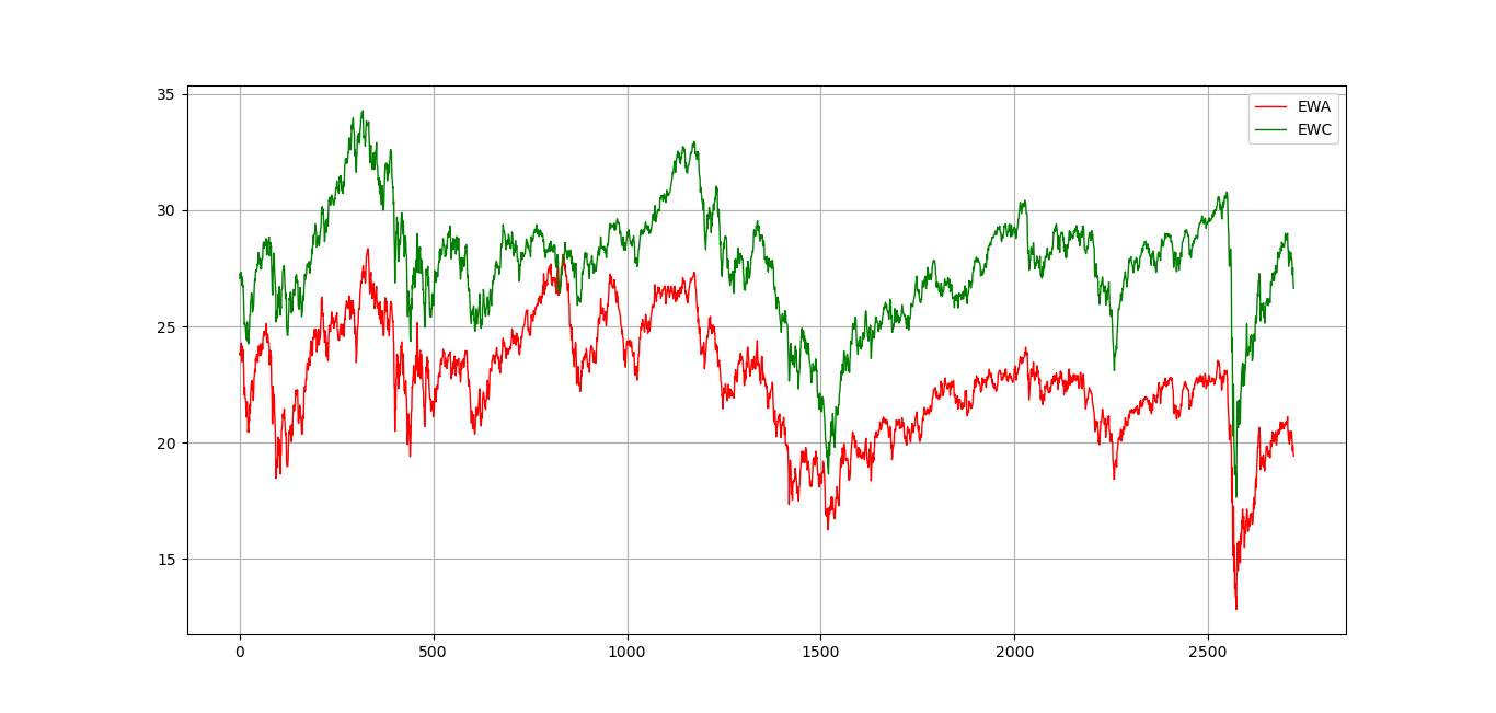
They do seem very correlated, but are they cointegrated? In other words, is their spread mean-reverting and stationary? That’s what we will be back-testing. If the series are indeed stationary then we will form a pairs trading simple strategy based on their spread (ignoring the hedge ratio). Let’s consider EWA to be Asset_2 variable and EWC to be Asset_1 variable in our code. The calculated correlation between the two seems to be the first unlocked door towards the strategy:

它们看起来确实很相关，但是它们是协整的吗？换句话说，它们的扩散是否是均值回归且平稳的？这就是我们将进行回测的内容。如果该系列确实是平稳的，那么我们将基于它们的价差(忽略对冲比率)形成一个交易简单策略的货币对。让我们在代码中将EWA视为Asset_2变量，将EWC视为Asset_1变量。两者之间的计算出的相关性似乎是通向该策略的第一个解锁门：

import numpy as np
np.corrcoef(Asset_1, Asset2)

The result we get will be around 0.85 which is a pretty strong linear correlation. Next, we will separately check whether the two time series are stationary or not, and then check if they are cointegrated or not. We will use statsmodels.tsa.stattools for the below.

我们得到的结果约为0.85，这是一个非常强的线性相关性。接下来，我们将分别检查两个时间序列是否稳定，然后检查它们是否协整。我们将在下面使用statsmodels.tsa.stattools。

def stationarity(a, cutoff = 0.05):
  a = np.ravel(a)
  if adfuller(a)[1] < cutoff:
    print(‘The series is stationary’)
    print(‘p-value = ‘, adfuller(a)[1])
  else:
    print(‘The series is NOT stationary’)
    print(‘p-value = ‘, adfuller(a)[1])stationarity(Asset_1)
stationarity(Asset_2)def cointegration(a, b):
  if coint(a, b)[1] < 0.05:
    print(‘The series are cointegrated’)
    print(‘p-value = ‘, coint(a, b)[1])
  else:
    print(‘The series are NOT cointegrated’)
    print(‘p-value = ‘, coint(a, b)[1])cointegration(Asset_1, Asset_2)

The above code will give these results. Naturally, we do not expect that these two random-like time series to be stationary (I just needed an excuse to provide the code) but what interests us is the result of the cointegration test which has a p-value of less than our chosen cut-off (5%), thus, rejecting the null hypothesis that there is no cointegration. Now, we have confirmation to back-test a strategy based on the two assets.

上面的代码将给出这些结果。自然，我们不希望这两个类似随机的时间序列是固定的(我只是需要一个借口来提供代码)，但是让我们感兴趣的是协整测试的结果，该协整测试的p值小于我们选择的p值截止(5％)，因此拒绝没有协整的原假设。现在，我们已经确认可以基于这两种资产对策略进行回测。

The series is NOT stationary (Asset_1):

系列不是固定的(Asset_1)：

p-value = 0.057

p值= 0.057

The series is NOT stationary (Asset_2):

系列不是固定的(Asset_2)：

p-value = 0.20

p值= 0.20

The series are cointegrated:

该系列是协整的：

p-value = 0.048

p值= 0.048

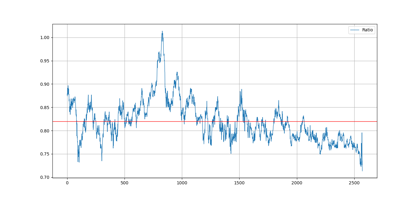
# Another check for stationarity in the ratio between the twoData[:, 2] = Asset_2 / Asset_1
Ratio = Data[:, 2]stationarity(Ratio)

When we calculate the ratio between the two and plot it we will have the next graph which seems to be mean-reverting. The spread seems to satisfy the stationarity test as well.

当我们计算两者之间的比率并将其绘制时，我们将得到下一个似乎均值回归的图形。价差似乎也满足了平稳性测试。

The series is stationary

该系列是固定的

p-value = 0.032

p值= 0.032

Now, we should standardize the ratio we have in order to normalize the signals.

现在，我们应该标准化比率以标准化信号。

# Standardization assuming the spreadfor i in range(len(Data)):
  try:
    Data[i, 3] = (Data[i — lookback:i + 1, 2].mean())
  except IndexError:
    pass# Calculating Standard deviationfor i in range(len(Data)):
  Data[i, 4] = ((Data[i — lookback:i + 1, 2].std()))# Standardizingfor i in range(len(Data)):
  Data[i, 5] = (Data[i, 2] — Data[i, 3]) / Data[i, 4]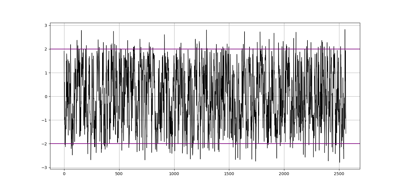

Main idea: We will back-test a dollar-neutral pairs trading strategy on the EWA and EWC ETFs. As we have explained above, the conditions of the back-test will be the following:

主要思想：我们将在EWA和EWC ETF上对美元中性货币对交易策略进行回测。如上文所述，回测的条件如下：

Holding period = 60
持有期= 60
Lookback period = 9
回溯期= 9
Upper barrier = 2
上限= 2
Lower barrier = -2
下屏障= -2

We can also use a variable period that relies on the when the mean reverts back to normality but in our back-test the holding period will be fixed.

我们还可以使用可变期间，该期间取决于均值恢复正常状态的时间，但在我们的回测中，保持期间将是固定的。

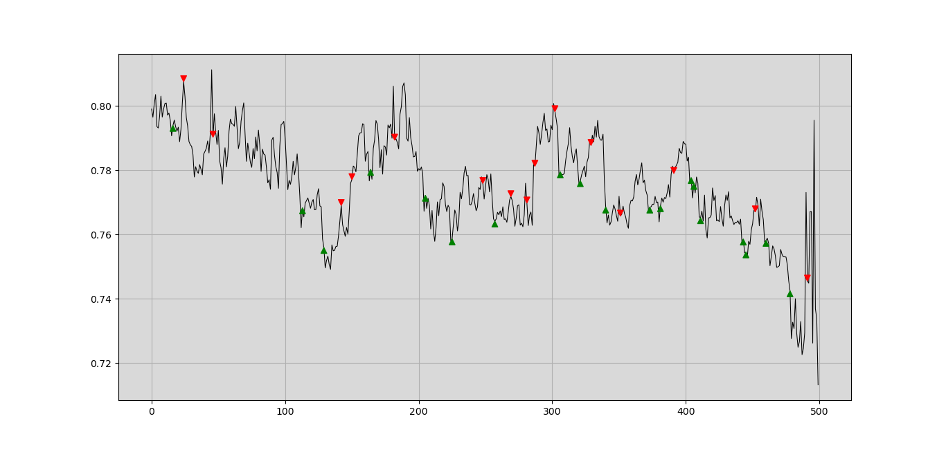
# Buy/Sell Conditionsfor i in range(len(Data)):
  try:
    if Data[i, 2] <= lower_barrier and Data[i — 1, 2] > lower_barrier:
      Data[i + 1, 4] = -1
      Data[i + 1, 5] = 1
    elif Data[i, 2] >= upper_barrier and Data[i — 1, 2] < upper_barrier:
      Data[i + 1, 6] = 1
      Data[i + 1, 7] = -1
    else:
      continue
  except IndexError:
    passfor i in range(len(Data)):
  try:
    if Data[i, 5] == 1:
      Data[i + holding_period, 8] = (Data[i + holding_period, 1] — Data[i, 1])
    if Data[i, 6] == 1:
      Data[i + holding_period, 8] = (Data[i + holding_period, 0] — Data[i, 0])
    if Data[i, 4] == -1:
      Data[i + holding_period, 9] = (Data[i, 0] — Data[i + holding_period, 0])
    if Data[i, 7] == -1:
      Data[i + holding_period, 9] = (Data[i, 1] — Data[i + holding_period, 1])
  except IndexError:
    pass

The next graph shows the equity curve from the strategy (gross of fees) and the results (assuming $1 investment with no leverage).

下一张图显示了该策略的权益曲线(费用总额)和结果(假设无杠杆的1美元投资)。

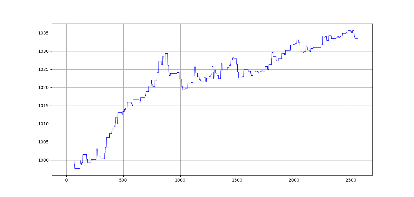
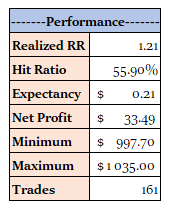
It is worth-mentioning again that the profit was only indicative as it is gross of fees and any other costs. Also, no leverage was used, so, the profit is not magnified which explains its weakness, but the strategy does seem to work even though we have a small bias by choosing the barriers and the lookback before starting.

再次值得一提的是，利润仅是指示性的，因为它是费用和任何其他费用的总额。同样，没有使用杠杆，因此利润没有被放大，这说明了它的弱点，但是即使我们在开始之前通过选择壁垒和回溯有小的偏见，该策略也确实有效。