


 本文介绍了如何使用PyOD库中的HBOS算法进行异常检测。通过生成toy example,展示了HBOS算法的工作原理,包括静态宽度和动态宽度直方图的构建,并解释了HBOS值的计算方式。实验结果显示,HBOS在训练数据和测试数据上的ROC曲线均为1,查准率@rank n达到1,表现出优秀的检测效果。
目标:使用PyOD库生成toy example并调用HBOS
- 使用pyod库生成toy example
官网上给出的代码为见pyod官网详细参数描述
pyod.utils.data.generate_data(n_train=1000, n_test=500, n_features=2, contamination=0.1, train_only=False, offset=10, behaviour='old', random_state=None)[source]
正态数据由多元高斯分布生成,离群值由均匀分布生成。返回值为
X_train (numpy array of shape (n_train, n_features)) – Training data.
y_train (numpy array of shape (n_train,)) – Training ground truth.
X_test (numpy array of shape (n_test, n_features)) – Test data.
y_test (numpy array of shape (n_test,)) – Test ground truth.
打印出来:

画图展示:
import numpy as np
import matplotlib.pyplot as plt
import pyod as py
dt=py.utils.data.generate_data(
        n_train=1000, n_test=500, n_features=2, contamination=0.1,
        train_only=False, offset=10, behaviour='old', random_state=None)
#对数据进行拆分
x_train=dt[0]
y_train=dt[1]
x_test=dt[2]
y_test=dt[3]
print(x_train)
print(y_train)
print(x_test)
F1=x_train[:,[0]].reshape(-1,1)
F2=x_train[:,[1]].reshape(-1,1)
f1=x_test[:,[0]].reshape(-1,1)
f2=x_test[:,[1]].reshape(-1,1)
plt.scatter(F1, F2,c = 'r',marker = 'o')
plt.scatter(f1, f2,c = 'b',marker = 'o')
plt.show()
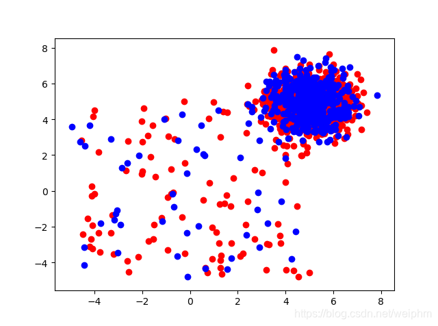
红色为train数据,紫色为test数据
2.调用HBOS
HBOS为频数直方图
HBOS算法流程:
- 为每个数据维度做出数据直方图。对分类数据统计每个值的频数并计算相对频率。对数值数据根据分布的不同采用以下两种方法:
静态宽度直方图:标准的直方图构建方法,在值范围内使用k个等宽箱。样本落入每个桶的频率(相对数量)作为密度(箱子高度)的估计。时间复杂度: O ( n ) O(n) O(n)
动态宽度直方图:首先对所有值进行排序,然后固定数量的 N k \frac{N}{k} kN个连续值装进一个箱里,其 中N是总实例数,k是箱个数;直方图中的箱面积表示实例数。因为箱的宽度是由箱中第一个值和最后一个值决定的,所有箱的面积都一样,因此每一个箱的高度都是可计算的。这意味着跨度大的箱的高度低,即密度小,只有一种情况例外,超过k个数相等,此时允许在同一个箱里超过 N k \frac{N}{k} kN值。
时间复杂度: O ( n × l o g ( n ) ) O(n\times log(n)) O(n×log(n))
- 对每个维度都计算了一个独立的直方图,其中每个箱子的高度表示密度的估计。然后为了使得最大高度为1(确保了每个特征与异常值得分的权重相等),对直方图进行归一化处理。最后,每一个实例的HBOS值由以下公式计算:
H
B
O
S
(
p
)
=
∑
i
=
0
d
log
(
1
hist
i
(
p
)
)
H B O S(p)=\sum_{i=0}^{d} \log \left(\frac{1}{\text {hist}_{i}(p)}\right)
HBOS(p)=i=0∑dlog(histi(p)1)
调用HBOS,不直接对py.utils.data.generate_data中的contamintation赋值
from pyod.models.hbos import HBOS
x_train,y_train,x_test,y_test=py.utils.data.generate_data(
        n_train=1000, n_test=500, n_features=2,
        train_only=False,behaviour='old',offset=10)
#对数据进行拆分
outlier_fraction = 0.1
x_outliers, x_inliers = py.utils.data.get_outliers_inliers(x_train,y_train)
n_inliers = len(x_inliers)
n_outliers = len(x_outliers)
#使用HBOS
classifiers = {
    'Histogram-base Outlier Detection (HBOS)': HBOS(contamination=outlier_fraction)}
3.看HBOS的分类效果
使用classifier拟合这些数据
from pyod.utils.example import visualize
from pyod.utils.data import evaluate_print
for i, (clf_name, clf) in enumerate(classifiers.items()):
    clf.fit(x_train)
    y_train_pred = clf.labels_  # binary labels (0: inliers, 1: outliers)
    y_train_scores = clf.decision_scores_  # raw outlier scores
# get the prediction on the test data
    y_test_pred = clf.predict(x_test)  # outlier labels (0 or 1)
    y_test_scores = clf.decision_function(x_test)  # outlier scores
    clf_name = 'HBOS'
    print("\nOn Training Data:")
    evaluate_print(clf_name, y_train, y_train_scores)
    print("\nOn Test Data:")
    evaluate_print(clf_name, y_test, y_test_scores)
    visualize(clf_name, x_train, y_train, x_test, y_test, y_train_pred,
     y_test_pred, show_figure=True, save_figure=False)
最终结果:
On Training Data:
HBOS ROC:0.995, precision @ rank n:1.0
On Test Data:
HBOS ROC:1.0, precision @ rank n:1.0
图像:
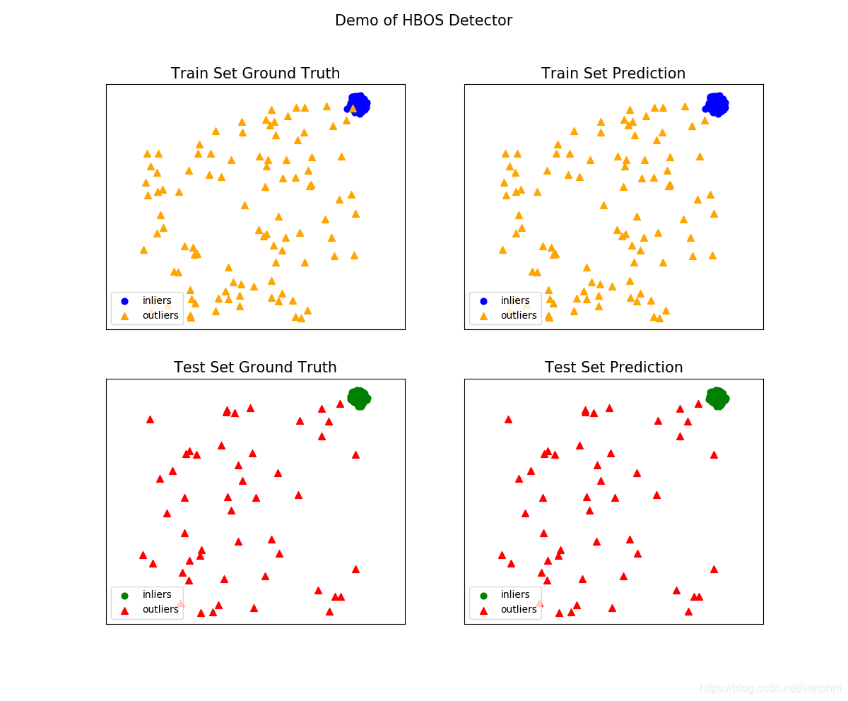
可以看到train集和test集上效果都很好;
evaluate_print评价的指标基于异常的分数决定的标签继而计算查准率,即precision @ rank n


 1484
1484

 被折叠的 条评论
为什么被折叠?
被折叠的 条评论
为什么被折叠?
 到【灌水乐园】发言


