Query Planning

Query Planning

► Table Of Contents

Overview

The best feature of SQL (in all its implementations, not just SQLite) is that it is a declarative language, not a procedural language. When programming in SQL you tell the system what you want to compute, not how to compute it. The task of figuring out the howis delegated to the query planner subsystem within the SQL database engine.

For any given SQL statement, there might be hundreds or thousands or even millions of different algorithms of performing the operation. All of these algorithms will get the correct answer, though some will run faster than others. The query planner is an AIthat tries to pick the fastest and most efficient algorithm for each SQL statement.

Most of the time, the query planner in SQLite does a good job. However, the query planner needs indices to work with. These indices must normally be added by programmers. Rarely, the query planner AI will make a suboptimal algorithm choice. In those cases, programmers may want to provide additional hints to help the query planner do a better job.

This document provides background information about how the SQLite query planner and query engine work. Programmers can use this information to help create better indexes, and provide hints to help the query planner when needed.

Additional information is provided in the SQLite query planner and next generation query planner documents.

1. Searching

1.1. Tables Without Indices

Most tables in SQLite consist of zero or more rows with a unique integer key (the rowid or INTEGER PRIMARY KEY) followed by content. (The exception is WITHOUT ROWID tables.) The rows are logically stored in order of increasing rowid. As an example, this article uses a table named "FruitsForSale" which relates various fruits to the state where they are grown and their unit price at market. The schema is this:

CREATE TABLE FruitsForSale( Fruit TEXT, State TEXT, Price REAL );

With some (arbitrary) data, such a table might be logically stored on disk as shown in figure 1:

 

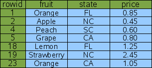
Figure 1: Logical Layout Of Table "FruitsForSale"

 

In this example, the rowids are not consecutive but they are ordered. SQLite usually creates rowids beginning with one and increasing by one with each added row. But if rows are deleted, gaps can appear in the sequence. And the application can control the rowid assigned if desired, so that rows are not necessarily inserted at the bottom. But regardless of what happens, the rowids are always unique and in strictly ascending order.

Suppose you want to look up the price of peaches. The query would be as follows:

SELECT price FROM fruitsforsale WHERE fruit='Peach';

To satisfy this query, SQLite reads every row out of the table, checks to see if the "fruit" column has the value of "Peach" and if so, outputs the "price" column from that row. The process is illustrated by figure 2 below. This is algorithm is called a full table scansince the entire content of the table must be read and examined in order to find the one row of interest. With a table of only 7 rows, a full table scan is acceptable, but if the table contained 7 million rows, a full table scan might read megabytes of content in order to find a single 8-byte number. For that reason, one normally tries to avoid full table scans.

 

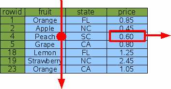
Figure 2: Full Table Scan

 

1.2. Lookup By Rowid

One technique for avoiding a full table scan is to do lookups by rowid (or by the equivalent INTEGER PRIMARY KEY). To lookup the price of peaches, one would query for the entry with a rowid of 4:

SELECT price FROM fruitsforsale WHERE rowid=4;

Since the information is stored in the table in rowid order, SQLite can find the correct row using a binary search. If the table contains N element, the time required to look up the desired row is proportional to logN rather than being proportional to N as in a full table scan. If the table contains 10 million elements, that means the query will be on the order of N/logN or about 1 million times faster.

 

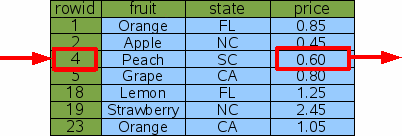
Figure 3: Lookup By Rowid

 

1.3. Lookup By Index

The problem with looking up information by rowid is that you probably do not care what the price of "item 4" is - you want to know the price of peaches. And so a rowid lookup is not helpful.

To make the original query more efficient, we can add an index on the "fruit" column of the "fruitsforsale" table like this:

CREATE INDEX Idx1 ON fruitsforsale(fruit);

An index is another table similar to the original "fruitsforsale" table but with the content (the fruit column in this case) stored in front of the rowid and with all rows in content order. Figure 4 gives a logical view of the Idx1 index. The "fruit" column is the primary key used to order the elements of the table and the "rowid" is the secondary key used to break the tie when two or more rows have the same "fruit". In the example, the rowid has to be used as a tie-breaker for the "Orange" rows. Notice that since the rowid is always unique over all elements of the original table, the composite key of "fruit" followed by "rowid" will be unique over all elements of the index.

 

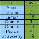
Figure 4: An Index On The Fruit Column

 

This new index can be used to implement a faster algorithm for the original "Price of Peaches" query.

SELECT price FROM fruitsforsale WHERE fruit='Peach';

The query starts by doing a binary search on the Idx1 index for entries that have fruit='Peach'. SQLite can do this binary search on the Idx1 index but not on the original FruitsForSale table because the rows in Idx1 are sorted by the "fruit" column. Having found a row in the Idx1 index that has fruit='Peach', the database engine can extract the rowid for that row. Then the database engines does a second binary search on the original FruitsForSale table to find the original row that contains fruit='Peach'. From the row in the FruitsForSale table, SQLite can then extract the value of the price column. This procedure is illustrated by figure 5.

 

Figure 5: Indexed Lookup For The Price Of Peaches

 

SQLite has to do two binary searches to find the price of peaches using the method show above. But for a table with a large number of rows, this is still much faster than doing a full table scan.

1.4. Multiple Result Rows

In the previous query the fruit='Peach' constraint narrowed the result down to a single row. But the same technique works even if multiple rows are obtained. Suppose we looked up the price of Oranges instead of Peaches:

SELECT price FROM fruitsforsale WHERE fruit='Orange'

 

Figure 6: Indexed Lookup For The Price Of Oranges

 

In this case, SQLite still does a single binary search to find the first entry of the index where fruit='Orange'. Then it extracts the rowid from the index and uses that rowid to lookup the original table entry via binary search and output the price from the original table. But instead of quitting, the database engine then advances to the next row of index to repeat the process for next fruit='Orange' entry. Advancing to the next row of an index (or table) is much less costly than doing a binary search since the next row is often located on the same database page as the current row. In fact, the cost of advancing to the next row is so cheap in comparison to a binary search that we usually ignore it. So our estimate for the total cost of this query is 3 binary searches. If the number of rows of output is K and the number of rows in the table is N, then in general the cost of doing the query is proportional to (K+1)*logN.

1.5. Multiple AND-Connected WHERE-Clause Terms

Next, suppose that you want to look up the price of not just any orange, but specifically California-grown oranges. The appropriate query would be as follows:

SELECT price FROM fruitsforsale WHERE fruit='Orange' AND state='CA'

 

Figure 7: Indexed Lookup Of California Oranges

 

One approach to this query is to use the fruit='Orange' term of the WHERE clause to find all rows dealing with oranges, then filter those rows by rejecting any that are from states other than California. This process is shown by figure 7 above. This is a perfectly reasonable approach in most cases. Yes, the database engine did have to do an extra binary search for the Florida orange row that was later rejected, so it was not as efficient as we might hope, though for many applications it is efficient enough.

Suppose that in addition to the index on "fruit" there was also an index on "state".

CREATE INDEX Idx2 ON fruitsforsale(state);

 

Figure 8: Index On The State Column

 

The "state" index works just like the "fruit" index in that it is a new table with an extra column in front of the rowid and sorted by that extra column as the primary key. The only difference is that in Idx2, the first column is "state" instead of "fruit" as it is with Idx1. In our example data set, there is more redundancy in the "state" column and so they are more duplicate entries. The ties are still resolved using the rowid.

Using the new Idx2 index on "state", SQLite has another option for lookup up the price of California oranges: it can look up every row that contains fruit from California and filter out those rows that are not oranges.

 

Figure 9: Indexed Lookup Of California Oranges

 

Using Idx2 instead of Idx1 causes SQLite to examine a different set of rows, but it gets the same answer in the end (which is very important - remember that indices should never change the answer, only help SQLite to get to the answer more quickly) and it does the same amount of work. So the Idx2 index did not help performance in this case.

The last two queries take the same amount of time, in our example. So which index, Idx1 or Idx2, will SQLite choose? If theANALYZE command has been run on the database, so that SQLite has had an opportunity to gather statistics about the available indices, then SQLite will know that the Idx1 index usually narrows the search down to a single item (our example of fruit='Orange' is the exception to this rule) whereas the Idx2 index will normally only narrow the search down to two rows. So, if all else is equal, SQLite will choose Idx1 with the hope of narrowing the search to as small a number of rows as possible. This choice is only possible because of the statistics provided by ANALYZE. If ANALYZE has not been run then the choice of which index to use is arbitrary.

1.6. Multi-Column Indices

To get the maximum performance out of a query with multiple AND-connected terms in the WHERE clause, you really want a multi-column index with columns for each of the AND terms. In this case we create a new index on the "fruit" and "state" columns of FruitsForSale:

CREATE INDEX Idx3 ON FruitsForSale(fruit, state);

 

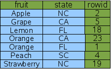
Figure 1: A Two-Column Index

 

A multi-column index follows the same pattern as a single-column index; the indexed columns are added in front of the rowid. The only difference is that now multiple columns are added. The left-most column is the primary key used for ordering the rows in the index. The second column is used to break ties in the left-most column. If there were a third column, it would be used to break ties for the first two columns. And so forth for all columns in the index. Because rowid is guaranteed to be unique, every row of the index will be unique even if all of the content columns for two rows are the same. That case does not happen in our sample data, but there is one case (fruit='Orange') where there is a tie on the first column which must be broken by the second column.

Given the new multi-column Idx3 index, it is now possible for SQLite to find the price of California oranges using only 2 binary searches:

SELECT price FROM fruitsforsale WHERE fruit='Orange' AND state='CA'

 

Figure 11: Lookup Using A Two-Column Index

 

With the Idx3 index on both columns that are constrained by the WHERE clause, SQLite can do a single binary search against Idx3 to find the one rowid for California oranges, then do a single binary search to find the price for that item in the original table. There are no dead-ends and no wasted binary searches. This is a more efficient query.

Note that Idx3 contains all the same information as the original Idx1. And so if we have Idx3, we do not really need Idx1 any more. The "price of peaches" query can be satisfied using Idx3 by simply ignoring the "state" column of Idx3:

SELECT price FROM fruitsforsale WHERE fruit='Peach'

 

Figure 12: Single-Column Lookup On A Multi-Column Index

 

Hence, a good rule of thumb is that your database schema should never contain two indices where one index is a prefix of the other. Drop the index with fewer columns. SQLite will still be able to do efficient lookups with the longer index.

1.7. Covering Indices

The "price of California oranges" query was made more efficient through the use of a two-column index. But SQLite can do even better with a three-column index that also includes the "price" column:

CREATE INDEX Idx4 ON FruitsForSale(fruit, state, price);

 

Figure 13: A Covering Index

 

This new index contains all the columns of the original FruitsForSale table that are used by the query - both the search terms and the output. We call this a "covering index". Because all of the information needed is in the covering index, SQLite never needs to consult the original table in order to find the price.

SELECT price FROM fruitsforsale WHERE fruit='Orange' AND state='CA';

 

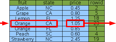
Figure 14: Query Using A Covering Index

 

Hence, by adding extra "output" columns onto the end of an index, one can avoid having to reference the original table and thereby cut the number of binary searches for a query in half. This is a constant-factor improvement in performance (roughly a doubling of the speed). But on the other hand, it is also just a refinement; A two-fold performance increase is not nearly as dramatic as the one-million-fold increase seen when the table was first indexed. And for most queries, the difference between 1 microsecond and 2 microseconds is unlikely to be noticed.

1.8. OR-Connected Terms In The WHERE Clause

Multi-column indices only work if the constraint terms in the WHERE clause of the query are connected by AND. So Idx3 and Idx4 are helpful when the search is for items that are both Oranges and grown in California, but neither index would be that useful if we wanted all items that were either oranges or are grown in California.

SELECT price FROM FruitsForSale WHERE fruit='Orange' OR state='CA';

When confronted with OR-connected terms in a WHERE clause, SQLite examines each OR term separately and tries to use an index to find the rowids associated with each term. It then takes the union of the resulting rowid sets to find the end result. The following figure illustrates this process:

 

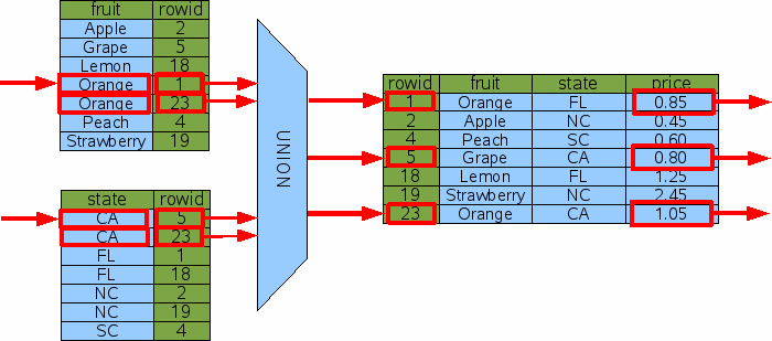
Figure 15: Query With OR Constraints

 

The diagram above implies that SQLite computes all of the rowids first and then combines them with a union operation before starting to do rowid lookups on the original table. In reality, the rowid lookups are interspersed with rowid computations. SQLite uses one index at a time to find rowids while remembering which rowids it has seen before so as to avoid duplicates. That is just an implementation detail, though. The diagram, while not 100% accurate, provides a good overview of what is happening.

In order for the OR-by-UNION technique shown above to be useful, there must be an index available that helps resolve every OR-connected term in the WHERE clause. If even a single OR-connected term is not indexed, then a full table scan would have to be done in order to find the rowids generated by the one term, and if SQLite has to do a full table scan, it might as well do it on the original table and get all of the results in a single pass without having to mess with union operations and follow-on binary searches.

One can see how the OR-by-UNION technique could also be leveraged to use multiple indices on queries where the WHERE clause has terms connected by AND, by using an intersect operator in place of union. Many SQL database engines will do just that. But the performance gain over using just a single index is slight and so SQLite does not implement that technique at this time. However, a future version SQLite might be enhanced to support AND-by-INTERSECT.

2. Sorting

SQLite (like all other SQL database engines) can also use indices to satisfy the ORDER BY clauses in a query, in addition to expediting lookup. In other words, indices can be used to speed up sorting as well as searching.

When no appropriate indices are available, a query with an ORDER BY clause must be sorted as a separate step. Consider this query:

SELECT * FROM fruitsforsale ORDER BY fruit;

SQLite processes this by gathering all the output of query and then running that output through a sorter.

 

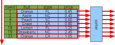
Figure 16: Sorting Without An Index

 

If the number of output rows is K, then the time needed to sort is proportional to KlogK. If K is small, the sorting time is usually not a factor, but in a query such as the above where K==N, the time needed to sort can be much greater than the time needed to do a full table scan. Furthermore, the entire output is accumulated in temporary storage (which might be either in main memory or on disk, depending on various compile-time and run-time settings) which can mean that a lot of temporary storage is required to complete the query.

2.1. Sorting By Rowid

Because sorting can be expensive, SQLite works hard to convert ORDER BY clauses into no-ops. If SQLite determines that output will naturally appear in the order specified, then no sorting is done. So, for example, if you request the output in rowid order, no sorting will be done:

SELECT * FROM fruitsforsale ORDER BY rowid;

 

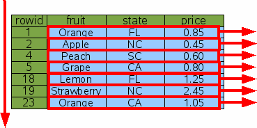
Figure 17: Sorting By Rowid

 

You can also request a reverse-order sort like this:

SELECT * FROM fruitsforsale ORDER BY rowid DESC;

SQLite will still omit the sorting step. But in order for output to appear in the correct order, SQLite will do the table scan starting at the end and working toward the beginning, rather than starting at the beginning and working toward the end as shown in figure 17.

2.2. Sorting By Index

Of course, ordering the output of a query by rowid is seldom useful. Usually one wants to order the output by some other column.

If an index is available on the ORDER BY column, that index can be used for sorting. Consider the request for all items sorted by "fruit":

SELECT * FROM fruitsforsale ORDER BY fruit;

 

Figure 18: Sorting With An Index

 

The Idx1 index is scanned from top to bottom (or from bottom to top if "ORDER BY fruit DESC" is used) in order to find the rowids for each item in order by fruit. Then for each rowid, a binary search is done to lookup and output that row. In this way, the output appears in the requested order without the need to gather the entire output and sort it using a separate step.

But does this really save time? The number of steps in the original indexless sort is proportional to NlogN since that is how much time it takes to sort N rows. But when we use Idx1 as shown here, we have to do N rowid lookups which take logN time each, so the total time of NlogN is the same!

SQLite uses a cost-based query planner. When there are two or more ways of solving the same query, SQLite tries to estimate the total amount of time needed to run the query using each plan, and then uses the plan with the lowest estimated cost. A cost is computed mostly from the estimated time, and so this case could go either way depending on the table size and what WHERE clause constraints were available, and so forth. But generally speaking, the indexed sort would probably be chosen, if for no other reason, because it does not need to accumulate the entire result set in temporary storage before sorting and thus uses much less temporary storage.

2.3. Sorting By Covering Index

If a covering index can be used for a query, then the multiple rowid lookups can be avoided and the cost of the query drops dramatically.

 

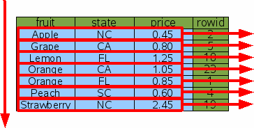
Figure 19: Sorting With A Covering Index

 

With a covering index, SQLite can simply walk the index from one end to the other and deliver the output in time proportional to N and without having allocate a large buffer to hold the result set.

3. Searching And Sorting At The Same Time

The previous discussion has treated searching and sorting as separate topics. But in practice, it is often the case that one wants to search and sort at the same time. Fortunately, it is possible to do this using a single index.

3.1. Searching And Sorting With A Multi-Column Index

Suppose we want to find the prices of all kinds of oranges sorted in order of the state where they are grown. The query is this:

SELECT price FROM fruitforsale WHERE fruit='Orange' ORDER BY state

The query contains both a search restriction in the WHERE clause and a sort order in the ORDER BY clause. Both the search and the sort can be accomplished at the same time using the two-column index Idx3.

 

Figure 20: Search And Sort By Multi-Column Index

 

The query does a binary search on the index to find the subset of rows that have fruit='Orange'. (Because the fruit column is the left-most column of the index and the rows of the index are in sorted order, all such rows will be adjacent.) Then it scans the matching index rows from top to bottom to get the rowids for the original table, and for each rowid does a binary search on the original table to find the price.

You will notice that there is no "sort" box anywhere in the above diagram. The ORDER BY clause of the query has become a no-op. No sorting has to be done here because the output order is by the state column and the state column also happens to be the first column after the fruit column in the index. So, if we scan entries of the index that have the same value for the fruit column from top to bottom, those index entries are guaranteed to be ordered by the state column.

3.2. Searching And Sorting With A Covering Index

A covering index can also be used to search and sort at the same time. Consider the following:

SELECT * FROM fruitforsale WHERE fruit='Orange' ORDER BY state

 

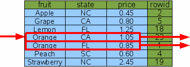
Figure 21: Search And Sort By Covering Index

 

As before, SQLite does single binary search for the range of rows in the covering index that satisfy the WHERE clause, the scans that range from top to bottom to get the desired results. The rows that satisfy the WHERE clause are guaranteed to be adjacent since the WHERE clause is an equality constraint on the left-most column of the index. And by scanning the matching index rows from top to bottom, the output is guaranteed to be ordered by state since the state column is the very next column to the right of the fruit column. And so the resulting query is very efficient.

SQLite can pull a similar trick for a descending ORDER BY:

SELECT * FROM fruitforsale WHERE fruit='Orange' ORDER BY state DESC

The same basic algorithm is followed, except this time the matching rows of the index are scanned from bottom to top instead of from top to bottom, so that the states will appear in descending order.

3.3. Partial Sorting Using An Index (a.k.a. Block Sorting)

Sometimes only part of an ORDER BY clause can be satisfied using indexes. Consider, for example, the following query:

SELECT * FROM fruitforsale ORDER BY fruit, price

If the covering index is used for the scan, the "fruit" column will appear naturally in the correct order, but when there are two or more rows with the same fruit, the price might be out of order. When this occurs, SQLite does many small sorts, one sort for each distinct value of fruit, rather than one large sort. Figure 22 below illustrates the concept.

 

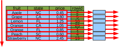
Figure 22: Partial Sort By Index

 

In the example, instead of a single sort of 7 elements, there are 5 sorts of one-element each and 1 sort of 2 elements for the case of fruit=='Orange'.

The advantages of doing many smaller sorts instead of a single large sort are:

1. Multiple small sorts collectively use fewer CPU cycles than a single large sort.
2. Each small sort is run independently, meaning that much less information needs to be kept in temporary storage at any one time.
3. Those columns of the ORDER BY that are already in the correct order due to indexes can be omitted from the sort key, further reducing storage requirements and CPU time.
4. Output rows can be returned to the application as each small sort completes, and well before the table scan is complete.
5. If a LIMIT clause is present, it might be possible to avoid scanning the entire table.

Because of these advantages, SQLite always tries to do a partial sort using an index even if a complete sort by index is not possible.

4. WITHOUT ROWID tables

The basic principals described above apply to both ordinary rowid tables and WITHOUT ROWID tables. The only difference is that the rowid column that serves as the key for tables and that appears as the right-most term in indexes is replaced by the PRIMARY KEY.