Tensorflow tflearn 编写RCNN（转+修改）

最新推荐文章于 2021-09-26 21:49:38 发布

原创最新推荐文章于 2021-09-26 21:49:38 发布 · 996 阅读

5 ·

CC 4.0 BY-SA版权

文章标签：

#RCNN

目标检测专栏收录该内容

16 篇文章

订阅专栏

原帖： http://www.cnblogs.com/edwardbi/p/5647522.html

原帖GitHub： https://github.com/edwardbi/DeepLearningModels/tree/master/RCNN

少量代码需要修改尤其是缩进的问题！！

修改后的Github:https://github.com/UncleLLD/RCNN/ 修改地方可以参考下，也许是自己的版本问题，有过一些报错。

最后以修改缩进以及python3版本运行完成重现

两周多的努力总算写出了RCNN的代码，这段代码非常有意思，并且还顺带复习了几个Tensorflow应用方面的知识点，故特此总结下，带大家分享下经验。理论方面，RCNN的理论教程颇多，这里我不在做详尽说明，有兴趣的朋友可以看看这个博客以了解大概。

系统概况

RCNN的逻辑基于Alexnet模型。为增加模型的物体辨识率，在图片未经CNN处理前，先由传统算法（文中所用算法为Selective Search算法）取得大概2000左右的疑似物品框。之后，这些疑似框被导入CNN系统中以取得输出层前一层的特征后，由训练好的svm来区分物体。这之中，比较有意思的部分包括了对经过ImageNet训练后的Alexnet的fine tune，对fine tune后框架里输出层前的最后一层特征点的提取以及训练svm分类器。下面，让我们来看看如何实现这个模型吧！

代码解析

为方便编写，这里应用了tflearn库作为tensorflow的一个wrapper来编写Alexnet，关于tflearn，具体资料请点击这里查看其官网。

那么下面，让我们先来看看系统流程：

第一步，训练Alexnet，这里我们运用的是github上tensorflow-alexnet项目。该项目将Alexnet运用在学习flower17数据库上，说白了也就是区分不同种类的花的项目。github提供的代码所有功能作者都有认真的写出，不过在main的写作以及对模型是否支持在断点处继续训练等问题上作者并没写明，这里贴上我的代码：

def train(network, X, Y):

# Training

model = tflearn.DNN(network, checkpoint_path='model_alexnet',

max_checkpoints=1, tensorboard_verbose=2, tensorboard_dir='output')

# 这里增加了读取存档的模式。如果已经有保存了的模型，我们当然就读取它然后继续

# 训练了啊！

if os.path.isfile('model_save.model'):

model.load('model_save.model')

model.fit(X, Y, n_epoch=100, validation_set=0.1, shuffle=True,

show_metric=True, batch_size=64, snapshot_step=200,

snapshot_epoch=False, run_id='alexnet_oxflowers17') # epoch = 1000

# Save the model

# 这里是保存已经运算好了的模型

model.save('model_save.model')

同时，我们希望可以检测模型是否运作正常。以下是检测Alexnet用代码

# 预处理图片函数：

# ------------------------------------------------------------------------------------------------

# 首先，读取图片，形成一个Image文件

def load_image(img_path):

img = Image.open(img_path)

return img

# 将Image文件给修改成224 * 224的图片大小（当然，RGB三个频道我们保持不变）

def resize_image(in_image, new_width, new_height, out_image=None,

resize_mode=Image.ANTIALIAS):

img = in_image.resize((new_width, new_height), resize_mode)

if out_image:

img.save(out_image)

return img

# 将Image加载后转换成float32格式的tensor

def pil_to_nparray(pil_image):

pil_image.load()

return np.asarray(pil_image, dtype="float32")

# 网络框架函数：

# ------------------------------------------------------------------------------------------------

def create_alexnet(num_classes):

# Building 'AlexNet'

network = input_data(shape=[None, 224, 224, 3])

network = conv_2d(network, 96, 11, strides=4, activation='relu')

network = max_pool_2d(network, 3, strides=2)

network = local_response_normalization(network)

network = conv_2d(network, 256, 5, activation='relu')

network = max_pool_2d(network, 3, strides=2)

network = local_response_normalization(network)

network = conv_2d(network, 384, 3, activation='relu')

network = conv_2d(network, 256, 3, activation='relu')

network = max_pool_2d(network, 3, strides=2)

network = local_response_normalization(network)

network = fully_connected(network, 4096, activation='tanh')

network = dropout(network, 0.5)

network = fully_connected(network, 4096, activation='tanh')

network = dropout(network, 0.5)

network = fully_connected(network, num_classes, activation='softmax')

network = regression(network, optimizer='momentum',

loss='categorical_crossentropy',

learning_rate=0.001)

return network

# 我们就是用这个函数来推断输入图片的类别的

def predict(network, modelfile,images):

model = tflearn.DNN(network)

model.load(modelfile)

return model.predict(images)

if __name__ == '__main__':

img_path = 'testimg7.jpg'

imgs = []

img = load_image(img_path)

img = resize_image(img, 224, 224)

imgs.append(pil_to_nparray(img))

net = create_alexnet(17)

predicted = predict(net, 'model_save.model',imgs)

print(predicted)

到此为止，我们跟RCNN还没有直接的关系。不过，值得注意的是，我们之前保存的那个训练模型model_save.model文件就是我们预训练的Alexnet。那么下面，我们开始正式制作RCNN系统了，让我们先编写传统的框架proposal代码吧。

鉴于文中运用的算法是selective search，对这个算法我个人没有太接触过，所以从头编写非常耗时。这里我偷了个懒，运用python现成的库selectivesearch去完成，那么，预处理代码的重心就在另一个概念上了，即IOU， interection or union概念。这个概念之所以在这里很有用是因为一张图片我们人为的去标注往往只为途中的某一样物体进行了标注，其余的我们全部算作背景了。在这个概念下，如果电脑一次性选择了许多可能物品框，我们如何决定哪个框对应这物体呢？对于完全不重叠的方框我们自然认为其标注的不是物体而是背景，但是对于那些重叠的方框怎么分类呢？我们这里便使用了IOU概念，即重叠数值超过一个阀门数值我们便将其标注为该物体类别，其他情况下我们均标注该方框为背景。更加详细的讲解请点击这里。

那么在代码上我们如何实现这个IOU呢？

# IOU Part 1

def if_intersection(xmin_a, xmax_a, ymin_a, ymax_a, xmin_b, xmax_b, ymin_b, ymax_b):

if_intersect = False

# 通过四条if来查看两个方框是否有交集。如果四种状况都不存在，我们视为无交集

if xmin_a < xmax_b <= xmax_a and (ymin_a < ymax_b <= ymax_a or ymin_a <= ymin_b < ymax_a):

if_intersect = True

elif xmin_a <= xmin_b < xmax_a and (ymin_a < ymax_b <= ymax_a or ymin_a <= ymin_b < ymax_a):

if_intersect = True

elif xmin_b < xmax_a <= xmax_b and (ymin_b < ymax_a <= ymax_b or ymin_b <= ymin_a < ymax_b):

if_intersect = True

elif xmin_b <= xmin_a < xmax_b and (ymin_b < ymax_a <= ymax_b or ymin_b <= ymin_a < ymax_b):

if_intersect = True

else:

return False

# 在有交集的情况下，我们通过大小关系整理两个方框各自的四个顶点，通过它们得到交集面积

if if_intersect == True:

x_sorted_list = sorted([xmin_a, xmax_a, xmin_b, xmax_b])

y_sorted_list = sorted([ymin_a, ymax_a, ymin_b, ymax_b])

x_intersect_w = x_sorted_list[2] - x_sorted_list[1]

y_intersect_h = y_sorted_list[2] - y_sorted_list[1]

area_inter = x_intersect_w * y_intersect_h

return area_inter

# IOU Part 2

def IOU(ver1, vertice2):

# vertices in four points

# 整理输入顶点

vertice1 = [ver1[0], ver1[1], ver1[0]+ver1[2], ver1[1]+ver1[3]]

area_inter = if_intersection(vertice1[0], vertice1[2], vertice1[1], vertice1[3], vertice2[0], vertice2[2], vertice2[1], vertice2[3])

# 如果有交集，计算IOU

if area_inter:

area_1 = ver1[2] * ver1[3]

area_2 = vertice2[4] * vertice2[5]

iou = float(area_inter) / (area_1 + area_2 - area_inter)

return iou

return False

之后，我们便可以在fine tune Alexnet时以0.5为IOU的threthold，并在训练SVM时以0.3为threthold。达成该思维的函数如下：

# Read in data and save data for Alexnet

def load_train_proposals(datafile, num_clss, threshold = 0.5, svm = False, save=False, save_path='dataset.pkl'):

train_list = open(datafile,'r')

labels = []

images = []

for line in train_list:

tmp = line.strip().split(' ')

# tmp0 = image address

# tmp1 = label

# tmp2 = rectangle vertices

img = skimage.io.imread(tmp[0])

# python的selective search函数

img_lbl, regions = selectivesearch.selective_search(img, scale=500, sigma=0.9, min_size=10)

candidates = set()

for r in regions:

# excluding same rectangle (with different segments)

# 剔除重复的方框

if r['rect'] in candidates:

continue

# 剔除太小的方框

if r['size'] < 220:

continue

# resize to 224 * 224 for input

# 重整方框的大小

proposal_img, proposal_vertice = clip_pic(img, r['rect'])

# Delete Empty array

# 如果截取后的图片为空，剔除

if len(proposal_img) == 0:

continue

# Ignore things contain 0 or not C contiguous array

x, y, w, h = r['rect']

# 长或宽为0的方框，剔除

if w == 0 or h == 0:

continue

# Check if any 0-dimension exist

# image array的dim里有0的，剔除

[a, b, c] = np.shape(proposal_img)

if a == 0 or b == 0 or c == 0:

continue

im = Image.fromarray(proposal_img)

resized_proposal_img = resize_image(im, 224, 224)

candidates.add(r['rect'])

img_float = pil_to_nparray(resized_proposal_img)

images.append(img_float)

# 计算IOU

ref_rect = tmp[2].split(',')

ref_rect_int = [int(i) for i in ref_rect]

iou_val = IOU(ref_rect_int, proposal_vertice)

# labels, let 0 represent default class, which is background

index = int(tmp[1])

if svm == False:

label = np.zeros(num_clss+1)

if iou_val < threshold:

label[0] = 1

else:

label[index] = 1

labels.append(label)

else:

if iou_val < threshold:

labels.append(0)

else:

labels.append(index)

if save:

pickle.dump((images, labels), open(save_path, 'wb'))

return images, labels

需要注意的是，这里输入参数的svm当为True时我们便不需要用one hot的方式表达label了。

在预处理了输入图片后，我们需要用预处理后的图片集来fine tune Alexnet。

# Use a already trained alexnet with the last layer redesigned

# 这里定义了我们的Alexnet的fine tune框架。按照原文，我们需要丢弃alexnet的最后一层，即softmax

# 然后换上一层新的softmax专门针对新的预测的class数+1(因为多出了个背景class)。具体方法为设

# restore为False，这样在最后一层softmax处，我不restore任何数值。

def create_alexnet(num_classes, restore=False):

# Building 'AlexNet'

network = input_data(shape=[None, 224, 224, 3])

network = conv_2d(network, 96, 11, strides=4, activation='relu')

network = max_pool_2d(network, 3, strides=2)

network = local_response_normalization(network)

network = conv_2d(network, 256, 5, activation='relu')

network = max_pool_2d(network, 3, strides=2)

network = local_response_normalization(network)

network = conv_2d(network, 384, 3, activation='relu')

network = conv_2d(network, 256, 3, activation='relu')

network = max_pool_2d(network, 3, strides=2)

network = local_response_normalization(network)

network = fully_connected(network, 4096, activation='tanh')

network = dropout(network, 0.5)

network = fully_connected(network, 4096, activation='tanh')

network = dropout(network, 0.5)

network = fully_connected(network, num_classes, activation='softmax', restore=restore)

network = regression(network, optimizer='momentum',

loss='categorical_crossentropy',

learning_rate=0.001)

return network

# 这里，我们的训练从已经训练好的alexnet开始，即model_save.model开始读取。在训练后，我们

# 将训练资料收录到fine_tune_model_save.model里

def fine_tune_Alexnet(network, X, Y):

# Training

model = tflearn.DNN(network, checkpoint_path='rcnn_model_alexnet',

max_checkpoints=1, tensorboard_verbose=2, tensorboard_dir='output_RCNN')

if os.path.isfile('fine_tune_model_save.model'):

print("Loading the fine tuned model")

model.load('fine_tune_model_save.model')

elif os.path.isfile('model_save.model'):

print("Loading the alexnet")

model.load('model_save.model')

else:

print("No file to load, error")

return False

model.fit(X, Y, n_epoch=10, validation_set=0.1, shuffle=True,

show_metric=True, batch_size=64, snapshot_step=200,

snapshot_epoch=False, run_id='alexnet_rcnnflowers2') # epoch = 1000

# Save the model

model.save('fine_tune_model_save.model')

运用这两个函数可完成对Alexnet的fine tune。到此为止，我们完成了对Alexnet的直接运用，接下来，我们需要读取alexnet最后一层特征并用以训练svm。那么，我们怎么取得图片的feature呢？方法很简单，我们减去输出层即可。代码如下：

# Use a already trained alexnet with the last layer redesigned

def create_alexnet(num_classes, restore=False):

# Building 'AlexNet'

network = input_data(shape=[None, 224, 224, 3])

network = conv_2d(network, 96, 11, strides=4, activation='relu')

network = max_pool_2d(network, 3, strides=2)

network = local_response_normalization(network)

network = conv_2d(network, 256, 5, activation='relu')

network = max_pool_2d(network, 3, strides=2)

network = local_response_normalization(network)

network = conv_2d(network, 384, 3, activation='relu')

network = conv_2d(network, 256, 3, activation='relu')

network = max_pool_2d(network, 3, strides=2)

network = local_response_normalization(network)

network = fully_connected(network, 4096, activation='tanh')

network = dropout(network, 0.5)

network = fully_connected(network, 4096, activation='tanh')

network = regression(network, optimizer='momentum',

loss='categorical_crossentropy',

learning_rate=0.001)

return network

在得到features后，我们需要训练SVM。为何要训练SVM呢？直接用CNN的softmax就好不就是么？这个问题在之前提及的博客里有提及。简而言之，SVM适用于小样本训练，这里这么做可以提高准确率。训练SVM的代码如下：

# Construct cascade svms

def train_svms(train_file_folder, model):

# 这里，我们将不同的训练集合分配到不同的txt文件里，每一个文件只含有一个种类

listings = os.listdir(train_file_folder)

svms = []

for train_file in listings:

if "pkl" in train_file:

continue

# 得到训练单一种类SVM的数据。

X, Y = generate_single_svm_train(train_file_folder+train_file)

train_features = []

for i in X:

feats = model.predict([i])

train_features.append(feats[0])

print("feature dimension")

print(np.shape(train_features))

# 这里建立一个Cascade的SVM以区分所有物体

clf = svm.LinearSVC()

print("fit svm")

clf.fit(train_features, Y)

svms.append(clf)

return svms

在识别物体的时候，我们该怎么做呢？首先，我们通过一下函数得到输入图片的疑似物体框：

def image_proposal(img_path):

img = skimage.io.imread(img_path)

img_lbl, regions = selectivesearch.selective_search(

img, scale=500, sigma=0.9, min_size=10)

candidates = set()

images = []

vertices = []

for r in regions:

# excluding same rectangle (with different segments)

if r['rect'] in candidates:

continue

if r['size'] < 220:

continue

# resize to 224 * 224 for input

proposal_img, proposal_vertice = prep.clip_pic(img, r['rect'])

# Delete Empty array

if len(proposal_img) == 0:

continue

# Ignore things contain 0 or not C contiguous array

x, y, w, h = r['rect']

if w == 0 or h == 0:

continue

# Check if any 0-dimension exist

[a, b, c] = np.shape(proposal_img)

if a == 0 or b == 0 or c == 0:

continue

im = Image.fromarray(proposal_img)

resized_proposal_img = resize_image(im, 224, 224)

candidates.add(r['rect'])

img_float = pil_to_nparray(resized_proposal_img)

images.append(img_float)

vertices.append(r['rect'])

return images, vertices

该过程与预处理中函数类似，不过更简单，因为我们不需要考虑对应的label了。之后，我们将这些图片一个一个的输入网络以得到相对输出（其实可以一起做，不过我的电脑总是kill了，可能是内存或者其他问题吧），最后，应用cascaded的SVM就可以得到预测结果了。

大家对于试验结果一定很好奇。以下结果是对比了Alexnet和RCNN的运行结果。

首先，让我们来看看对于以下图片的结果：

对它的分析结果如下：在Alexnet的情况下，得到了以下数据：

判断为第四类花。实际结果在flower 17数据库中是最后一类，也就是第17类花。这里，第17类花的可能性仅次于第四类，为34%。那么，RCNN的结果如何呢？我们看下图：

显而易见，RCNN的正确率（1类）非常之高。

下面是本人的实践过程：

1.环境: Tensorflow version 0.7.1. Python version 2.7 ，scikit-learn dev distribution package.以及安装 tflearn（ github at https://github.com/tflearn/tflearn），还记得要安装 selective search , pip install selectivesearch.

Training Input: 17 flowers 数据集下载: https://github.com/ck196/tensorflow-alexnet. 下载完毕后将数据集保存到本文GitHub位置处作为网络的预训练数据。

2.运行代码：终端目录进入github文件

1.运行train_alexnet.py 训练alexnet网络，会生成model_save.model等文件，注意由于tf的版本不同，生成的文件数量也不一样，大致都是model文件

2.运行fine_tune_RCNN.py文件,使用文件夹中自带的2flowers数据库微调，按照原作者的代码，这里会报错no file to load, error。在看相关解答后

原因是tflearn的save模型在tensorflow最新版本上无法正确保存成tflearn文件，而是保存成了三个文件（.data-0000-of-00001/index/meta）。
将fine_tune_RCNN中的fine_tune_Alexnet函数进行如下修改，会运行成功。
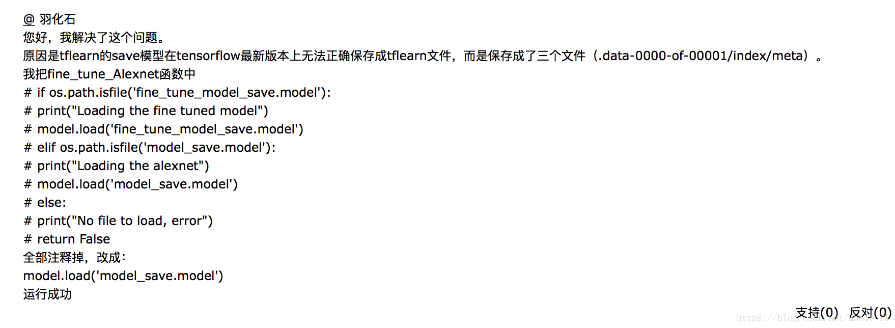
3.运行RCNN_output.py文件分类图像