


 本文详细解析了循环神经网络(RNN)中的反向传播通过时间(BPTT)算法,并探讨了其与传统反向传播的区别。同时,文章深入分析了梯度消失问题,并介绍了LSTM和GRU两种解决该问题的有效模型。
Note: RECURRENT NEURAL NETWORKS TUTORIAL, PART 3 – BACKPROPAGATION THROUGH TIME AND VANISHING GRADIENTS
本教程包括以下几个部分
1.Introduction To RNNs
2.Implementing a RNN using Python and Theano
3.Understanding the Backpropagation Through Time (BPTT) algorithm and the vanishing gradient problem
4.Implementing a GRU/LSTM RNN
翻译完发现这篇博客http://blog.youkuaiyun.com/rtygbwwwerr/article/details/51012699推导特别清楚,准备再整理一遍。
本文主要讨论BPTT的基本原理及与传统反向传播的区别。之后会讨论梯度消失问题,从而引入LSTM和GRUs(两大NLP神器)。梯度消失问题由Sepp Hochreiter于1991年首次发现,随着深度架构的应用而被重视起来。
理解本教程需要熟悉偏微分和反向传播策略。tutorial here and here and here。
BPTT
符号小换一下:
o
->
sty^t=tanh(Uxt+Wst−1)=softmax(Vst)
我们定义我们的loss(error),为交叉熵损失:
Et(yt,y^t)E(y,y^)=−ytlogy^t=∑tEt(yt,y^t)=−∑tytlogy^t
yt
是t时刻正确的单词,
y^t
是我们预测词。我们将一个句子看做一个训练对象,因此总error是每步的error之和。
梯度之和:
∂E∂W=∑t∂Et∂W
采用微分链式法则。以
E3
为例。
∂E3∂V=∂E3∂y^3∂y^3∂V=∂E3∂y^3∂y^3∂z3∂z3∂V=(y^3−y3)⊗s3
上式,
z3=Vs3
,
⊗
是向量外积。
∂E3∂V
只取决于当前step的值,即
y^3,y3,s3
。这样计算V的梯度就是一个矩阵乘法了。
对于W和U的求导就不一样了。
∂E3∂W=∂E3∂y^3∂y^3∂s3∂s3∂W
注意
s3=tanh(Uxt+Ws2)
与
s2
相关,其又依赖于W和
s1
等等。
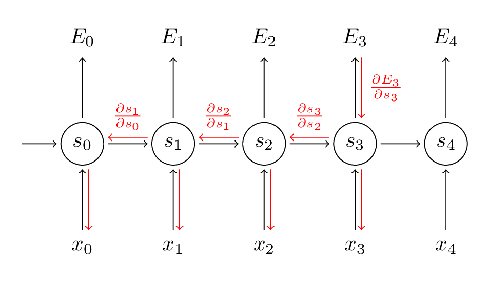
∂E3∂W=∑k=03∂E3∂y^3∂y^3∂s3∂s3∂sk∂sk∂W
我们把每一步的贡献都加起来给梯度。也就是,反向传播梯度求导时就要一直到t=0。
我们定义一个delta向量,这部分推导过程可参考此处。
δ(3)2=∂E3∂z2=∂E3∂s3∂s3∂s2∂s3∂z2
其中
z2=Ux2+Ws1
,(这里的
z2
就是隐层
s2
的输入)。应用到链式中
上代码:
def bptt(self, x, y):
    T = len(y)
    # Perform forward propagation
    o, s = self.forward_propagation(x)
    # We accumulate the gradients in these variables
    dLdU = np.zeros(self.U.shape)
    dLdV = np.zeros(self.V.shape)
    dLdW = np.zeros(self.W.shape)
    delta_o = o
    #这是delta求导的结果
    delta_o[np.arange(len(y)), y] -= 1.
    # For each output backwards...
    for t in np.arange(T)[::-1]:
        dLdV += np.outer(delta_o[t], s[t].T)
        # Initial delta calculation: dL/dz
        delta_t = self.V.T.dot(delta_o[t]) * (1 - (s[t] ** 2))
        # Backpropagation through time (for at most self.bptt_truncate steps)
        for bptt_step in np.arange(max(0, t-self.bptt_truncate), t+1)[::-1]:
            # print "Backpropagation step t=%d bptt step=%d " % (t, bptt_step)
            # Add to gradients at each previous step
            dLdW += np.outer(delta_t, s[bptt_step-1])
            dLdU[:,x[bptt_step]] += delta_t
            # Update delta for next step dL/dz at t-1
            delta_t = self.W.T.dot(delta_t) * (1 - s[bptt_step-1] ** 2)
    return [dLdU, dLdV, dLdW]
从这里可以看出,标准的RNN很难训练,序列会非常长,反向传播会经过很多层。
参考博客
http://www.wildml.com/2015/09/recurrent-neural-networks-tutorial-part-1-introduction-to-rnns/
http://blog.youkuaiyun.com/rtygbwwwerr/article/details/51012699


 11万+
11万+

 被折叠的 条评论
为什么被折叠?
被折叠的 条评论
为什么被折叠?
 到【灌水乐园】发言


