EEG 功能连接测量指标 | PLI / wPLI / dPLI

注：本文为 “EEG 功能连接测量指标” 相关合辑。
英文引文，机翻未校。
中文引文，略作重排。
如有内容异常，请看原文。

---

Comparing PLI, wPLI, and dPLI — MNE-Connectivity documentation
比较 PLI、wPLI 和 dPLI — MNE-Connectivity 文档

Note
注意

This example demonstrates the different connectivity information captured by the phase lag index (PLI) [1], weighted phase lag index (wPLI) [2], and directed phase lag index (dPLI) [3] on simulated data.
本示例展示了相位滞后指数（PLI）[1]、加权相位滞后指数（wPLI）[2] 和有向相位滞后指数（dPLI）[3] 在模拟数据上捕获的不同连接信息。

# Authors: Kenji Marshall <kenji.marshall99@gmail.com>
#          Charlotte Maschke <charlotte.maschke@mail.mcgill.ca>
#          Stefanie Blain-Moraes <stefanie.blain-moraes@mcgill.ca>
#
# License: BSD (3-clause)

import matplotlib.pyplot as plt
import mne
import numpy as np
from mne.datasets import sample

from mne_connectivity import spectral_connectivity_epochs

Background

背景

The formulae for PLI, wPLI, and dPLI are given below. In these equations, $S_{xy}$ is the cross-spectral density (CSD) between two signals $x$ and $y$. Importantly, the imaginary component of the CSD is maximal when the signals have a phase difference given by $\frac{\pi }{2}$, and is 0 when the phase difference is given by $\pi$ (where $k$ is an integer). This property provides protection against recognizing volume conduction effects as connectivity, and is the backbone for these methods [2]. In the equations below, $\text{Im}$ refers to the imaginary component, $H$ refers to the Heaviside step function, and $\text{sign}$ refers to the sign function.
PLI、wPLI 和 dPLI 的公式如下。在这些公式中，$S_{xy}$ 是两个信号 $x$ 和 $y$ 之间的互谱密度（CSD）。重要的是，当信号的相位差为 $\frac{\pi }{2}$ 时，CSD 的虚部达到最大值，而当相位差为 $\pi$（其中 $k$ 为整数）时，虚部为 0。这一特性可以防止将体积传导效应误认为是连接性，是这些方法的基本 [2]。在下面的公式中，$\text{Im}$ 表示虚部，$H$ 表示单位阶跃函数，$\text{sign}$ 表示符号函数。

$\text{PLI}=\left|\frac{\text{Im}(S_{xy})}{|\text{Im}(S_{xy})|}\right|$

$\text{wPLI}=\frac{|\text{Im}(S_{xy})|}{\text{Im}(S_{xy})+|\text{Im}(S_{xy})|}$

$\text{dPLI}=H(\text{Im}(S_{xy}))\cdot \text{sign}(\text{Im}(S_{xy}))$

All three of these metrics are bounded in the range ([0, 1]).
所有这三个指标都限制在 ([0, 1]) 范围内。

• For PLI, 0 means that signal $x$ leads and lags signal $y$ equally often, while a value greater than 0 means that there is an imbalance in the likelihood for signal $x$ to be leading or lagging. A value of 1 means that signal $x$ only leads or only lags signal $y$.
  对于 PLI，0 表示信号 $x$ 与信号 $y$ 的领先和滞后次数相等，而大于 0 的值则表示信号 $x$ 领先或滞后的可能性存在不平衡。值为 1 表示信号 $x$ 仅领先或仅滞后于信号 $y$。

• For wPLI, 0 means that the total weight (not the quantity) of all leading relationships equals the total weight of lagging relationships, while a value greater than 0 means that there is an imbalance between these weights. A value of 1, just as in PLI, means that signal $x$ only leads or only lags signal $y$.
  对于 wPLI，0 表示所有领先关系的总权重（而非数量）等于所有滞后关系的总权重，而大于 0 的值则表示这些权重之间存在不平衡。与 PLI 一样，值为 1 表示信号 $x$ 仅领先或仅滞后于信号 $y$。

• With dPLI, we gain the ability to distinguish whether signal $x$ is leading or lagging signal $y$, complementing the information provided by PLI or wPLI. A value of 0.5 means that signal $x$ leads and lags signal $y$ equally often. A value in the range ([0.5, 1]) means that signal $x$ leads signal $y$ more often than it lags, with a value of 1 meaning that signal $x$ always leads signal $y$. A value in the range ([0, 0.5)) means that signal $x$ lags signal $y$ more often than it leads, with a value of 0 meaning that signal $x$ always lags signal $y$. The PLI can actually be extracted from the dPLI by the relationship $\text{PLI}=2\cdot \text{dPLI}-1$, but this relationship is not invertible (dPLI cannot be estimated from the PLI).
  通过 dPLI，我们能够区分信号 $x$ 是领先还是滞后于信号 $y$，从而补充了 PLI 或 wPLI 提供的信息。值为 0.5 表示信号 $x$ 与信号 $y$ 的领先和滞后次数相等。范围在 ([0.5, 1]) 内的值表示信号 $x$ 领先于信号 $y$ 的次数多于滞后次数，值为 1 表示信号 $x$ 总是领先于信号 $y$。范围在 ([0, 0.5)) 内的值表示信号 $x$ 滞后于信号 $y$ 的次数多于领先次数，值为 0 表示信号 $x$ 总是滞后于信号 $y$。实际上，可以通过关系 $\text{PLI}=2\cdot \text{dPLI}-1$ 从 dPLI 中提取 PLI，但这种关系是不可逆的（无法从 PLI 估计 dPLI）。

Overall, these different approaches are closely related but have subtle differences, as will be demonstrated throughout the rest of this example.
总的来说，这些不同的方法密切相关，但存在细微的差别，这将在本示例的其余部分中展示。

Capturing Leading/Lagging Phase Relationships with dPLI
利用 dPLI 捕获领先/滞后的相位关系

The main advantage of dPLI is that it’s directed, meaning it can differentiate between phase relationships which are leading or lagging. To illustrate this, we generate sinusoids with Gaussian noise. In particular, we generate signals with phase differences of $0,-\pi ,-\frac{\pi }{2},0,\frac{\pi }{2},\pi$ relative to a reference signal. A negative difference means that the reference signal is lagging the other signal.
dPLI 的主要优势在于它是“有向的”，即可以区分领先或滞后的相位关系。为了说明这一点，我们生成带有高斯噪声的正弦波。具体来说，我们生成的信号与参考信号的相位差分别为 $0,-\pi ,-\frac{\pi }{2},0,\frac{\pi }{2},\pi$。负相位差表示参考信号滞后于其他信号。

fs = 250  # sampling rate (Hz)
n_e = 300  # number of epochs
T = 10  # length of epochs (s)
f = 10  # frequency of sinusoids (Hz)
t = np.arange(0, T, 1 / fs)
A = 1  # noise amplitude
sigma = 0.5  # Gaussian noise variance

data = []

phase_differences = [0, -np.pi, -np.pi / 2, 0, np.pi / 2, np.pi]
for ps in zip(phase_differences):
    sig = []
    for _ in range(n_e):
        sig.append(
            np.sin(2 * np.pi * f * t - ps)
            + A * np.random.normal(0, sigma, size=t.shape)
        )
    data.append(sig)

data = np.swapaxes(np.array(data), 0, 1)  # make epochs the first dimension

A snippet of this simulated data is shown below. The blue signal is the reference signal.
以下是模拟数据的一部分。蓝色信号是参考信号。

fig, ax = plt.subplots(1, 2, figsize=(12, 5), sharey=True)
ax[0].plot(t[:fs], data[0, 0, :fs], label="Reference")
ax[0].plot(t[:fs], data[0, 2, :fs])

ax[0].set_title(r"Phase Lagging ($-\pi/2$ Phase Difference)")
ax[0].set_xlabel("Time (s)")
ax[0].set_ylabel("Signal")
ax[0].legend()

ax[1].plot(t[:fs], data[0, 0, :fs], label="Reference")
ax[1].plot(t[:fs], data[0, 4, :fs])
ax[1].set_title(r"Phase Leading ($\pi/2$ Phase Difference)")
ax[1].set_xlabel("Time (s)")

plt.show()

We will now compute PLI, wPLI, and dPLI for each phase relationship.
接下来，我们将为每种相位关系计算 PLI、wPLI 和 dPLI。

conn = []
indices = ([0, 0, 0, 0, 0], [1, 2, 3, 4, 5])
for method in ["pli", "wpli", "dpli"]:
    conn.append(
        spectral_connectivity_epochs(
            data,
            method=method,
            sfreq=fs,
            indices=indices,
            fmin=9,
            fmax=11,
            faverage=True,
        ).get_data()[:, 0]
    )
conn = np.array(conn)

The estimated connectivites are shown in the figure below, which provides insight into the differences between PLI/wPLI, and dPLI.
估计的连接性如下面的图所示，它揭示了 PLI/wPLI 与 dPLI 之间的差异。

Similarities Of All Measures

所有指标的相似之处

• Capture presence of connectivity in same situations (phase difference of $\frac{\pi }{2}$)
  在相同情况下（相位差为 $\frac{\pi }{2}$）捕获连接性的存在

• Do not predict connectivity when phase difference is a multiple of $\pi$
  当相位差是 $\pi$ 的倍数时，不预测连接性

• Bounded between 0 and 1
  限制在 0 和 1 之间

How dPLI is Different Than PLI/wPLI

dPLI 与 PLI/wPLI 的不同之处

• Null connectivity is 0 for PLI and wPLI, but 0.5 for dPLI
  对于 PLI 和 wPLI，无连接性为 0，而对于 dPLI 为 0.5

• dPLI differentiates whether the reference signal is leading or lagging the other signal (lagging if $<0.5$, leading if $>0.5$)
  dPLI 可以区分参考信号是领先还是滞后于其他信号（如果 $<0.5$ 则表示滞后，如果 $>0.5$ 则表示领先）

x = np.arange(5)

plt.figure()
plt.bar(x - 0.2, conn[0], 0.2, align="center", label="PLI")
plt.bar(x, conn[1], 0.2, align="center", label="wPLI")
plt.bar(x + 0.2, conn[2], 0.2, align="center", label="dPLI")

plt.title("Connectivity Estimation Comparison")
plt.xticks(x, (r"$-\pi$", r"$-\pi/2$", r"$0$", r"$\pi/2$", r"$\pi$"))
plt.legend()
plt.xlabel("Phase Difference")
plt.ylabel("Estimated Connectivity")

plt.show()

Robustness to Outliers and Noise with wPLI

wPLI 对异常值和噪声的鲁棒性

The previous experiment illustrated the advantages conferred by dPLI when differentiating leading and lagging phase relationships. This experiment will now focus on understanding the advantages of wPLI, and explore how it extends upon PLI.
前面的实验展示了 dPLI 在区分领先和滞后相位关系时的优势。接下来的实验将重点关注 wPLI 的优势，并探讨它是如何扩展 PLI 的。

The main difference between PLI and wPLI is in how different phase relationships are weighted. In PLI, phase differences are weighted as 1 or -1 according to their sign. In wPLI, phase differences are weighted based on their value, meaning that phase differences closer to $\frac{\pi }{2}$ are weighted more heavily than those close to 0 or any other multiple of $\pi$.
PLI 和 wPLI 的主要区别在于不同相位关系的_权重_。在 PLI 中，根据相位差的符号将其权重设置为 1 或 -1。而在 wPLI 中，根据相位差的值来分配权重，即相位差越接近 $\frac{\pi }{2}$，其权重就越大，而接近 0 或 $\pi$ 的倍数的相位差则权重较小。

This avoids a discontinuity at the transition between positive and negative phase, treating all phase differences near this transition in a similar way. This provides some robustness against outliers and noise when estimating connectivity. For instance, volume conduction can distort EEG/MEG recordings, wherein signals emanating from the same neural source will be picked up by multiple sensors on the scalp. This can effect connectivity estimations, bringing the relative phase differences between two signals close to 0. wPLI minimizes the contribution of phase relationships that are small but non-zero (and may thus be attributed to volume conduction), while PLI weighs these in the same way as phase relationships of $\frac{\pi }{2}$.
这种方法避免了正相位和负相位之间的不连续性，将所有接近这一转换的相位差以类似的方式处理。这在估计连接性时对异常值和噪声具有一定的鲁棒性。例如，体积传导可能会扭曲 EEG/MEG 记录，来自同一神经源的信号会被头皮上的多个传感器捕捉到。这会影响连接性估计，使两个信号之间的相对相位差接近 0。wPLI 最小化了小但非零的相位关系的贡献（这些可能归因于体积传导），而 PLI 则将这些相位关系与 $\frac{\pi }{2}$ 的相位关系同等对待。

To demonstrate this, we recreate a result from (Vinck et al, 2011) [2]. Two sinusoids are simulated, where the phase difference for half of the epochs is $\frac{\pi }{100}$, and is $\frac{\pi }{2}$ for the others. We also explore the effect of applying uniform noise to this phase difference.
为了说明这一点，我们重现了 (Vinck et al, 2011) [2] 中的一个结果。我们模拟了两个正弦波，其中一半的试验中相位差为 $\frac{\pi }{100}$，另一半试验中相位差为 $\frac{\pi }{2}$。我们还探讨了将均匀噪声应用于这种相位差的效果。

n_noise = 41  # amount of noise amplitude samples in [0, 4]
data = [[]]

# Generate reference
for _ in range(n_e):
    data[0].append(np.sin(2 * np.pi * f * t))

A_list = np.linspace(0, 4, n_noise)

for A in A_list:
    sig = []
    # Generate other signal
    for _ in range(int(n_e / 2)):  # phase difference -pi/100
        sig.append(
            np.sin(2 * np.pi * f * t + np.pi / 100 + A * np.random.uniform(-1, 1))
        )
    for _ in range(int(n_e / 2), n_e):  # phase difference pi/2
        sig.append(np.sin(2 * np.pi * f * t - np.pi / 2 + A * np.random.uniform (-1, 1)))
    data.append(sig)

data = np.swapaxes(np.array(data), 0, 1)

# Visualize the data
fig, ax = plt.subplots(1, 2, figsize=(12, 5), sharey=True)
ax[0].plot(t[:10], data[0, 0, :10], label="Reference")
ax[0].plot(t[:10], data[1, 1, :10])

ax[0].set_title(r"Phase Lagging ($-\pi/100$ Phase Difference)")
ax[0].set_xlabel("Time (s)")
ax[0].set_ylabel("Signal")
ax[0].legend()

ax[1].plot(t[:fs], data[0, 0, :fs], label="Reference")
ax[1].plot(t[:fs], data[-1, 1, :fs])
ax[1].set_title(r"Phase Leading ($\pi/2$ Phase Difference)")
ax[1].set_xlabel("Time (s)")

plt.show()

We can now compute PLI and wPLI
现在我们可以计算 PLI 和 wPLI

conn = []
indices = ([0] * n_noise, np.arange(1, n_noise + 1))
for method in ["pli", "wpli"]:
    conn.append(
        spectral_connectivity_epochs(
            data,
            method=method,
            sfreq=fs,
            indices=indices,
            fmin=9,
            fmax=11,
            faverage=True,
        ).get_data()[:, 0]
    )
conn = np.array(conn)

The results from the simulation are shown in the figure below. In the case without noise, the difference between wPLI and PLI is made obvious. In PLI, no connectivity is detected, as the $\frac{\pi }{100}$ phase differences are weighted in the exact same way as the $\frac{\pi }{2}$ relationships. wPLI is able to avoid the cancellation of the $\frac{\pi }{100}$ relationships.
模拟结果如下面的图所示。在没有噪声的情况下，wPLI 和 PLI 之间的差异显而易见。在 PLI 中，没有检测到连接性，因为 $\frac{\pi }{100}$ 的相位差与 $\frac{\pi }{2}$ 的关系被赋予了相同的权重。wPLI 能够避免 $\frac{\pi }{100}$ 关系的抵消。

As noise gets added, PLI increases since the $\frac{\pi }{2}$ relationships are made positive more often than the $\frac{\pi }{100}$ relationships are made negative. However, wPLI maintains an advantage in its ability to distinguish the underlying structure. Beyond a certain point, the noise dominates any pre-defined structure, and both methods behave similarly, tending toward 0. For a more detailed analysis of this result and the properties of wPLI, please refer to (Vinck et al, 2011) [2].
随着噪声的增加，PLI 增加了，因为 $\frac{\pi }{2}$ 的关系比 $\frac{\pi }{100}$ 的关系更频繁地变为正。然而，wPLI 在区分潜在结构方面仍然具有优势。在某个点之后，噪声会主导任何预定义的结构，两种方法的行为变得相似，趋向于 0。对于这一结果的详细分析以及 wPLI 的特性，请参阅 (Vinck et al, 2011) [2]。

Demo On MEG Data

在 MEG 数据上的演示

To finish this example, we also quickly demonstrate these methods on some sample MEG data recorded during visual stimulation.
为了完成这个示例，我们还在一些在视觉刺激期间记录的样本 MEG 数据上快速演示了这些方法。

data_path = sample.data_path()
raw_fname = data_path / "MEG/sample/sample_audvis_filt-0-40_raw.fif"
event_fname = data_path / "MEG/sample/sample_audvis_filt-0-40_raw-eve.fif"
raw = mne.io.read_raw_fif(raw_fname)
events = mne.read_events(event_fname)

# Select gradiometers
picks = mne.pick_types(
    raw.info, meg="grad", eeg=False, stim=False, eog=True, exclude="bads"
)

# Create epochs
event_id, tmin, tmax = 3, -0.2, 1.5  # need a long enough epoch for 5 cycles
epochs = mne.Epochs(
    raw,
    events,
    event_id,
    tmin,
    tmax,
    picks=picks,
    baseline=(None, 0),
    reject=dict(grad=4000e-13, eog=150e-6),
)
epochs.load_data().pick_types(meg="grad")  # just keep MEG and no EOG now

fmin, fmax = 4.0, 9.0  # compute connectivity within 4-9 Hz
sfreq = raw.info["sfreq"]  # the sampling frequency
tmin = 0.0  # exclude the baseline period

# Compute PLI, wPLI, and dPLI
con_pli = spectral_connectivity_epochs(
    epochs,
    method="pli",
    mode="multitaper",
    sfreq=sfreq,
    fmin=fmin,
    fmax=fmax,
    faverage=True,
    tmin=tmin,
    mt_adaptive=False,
    n_jobs=1,
)

con_wpli = spectral_connectivity_epochs(
    epochs,
    method="wpli",
    mode="multitaper",
    sfreq=sfreq,
    fmin=fmin,
    fmax=fmax,
    faverage=True,
    tmin=tmin,
    mt_adaptive=False,
    n_jobs=1,
)

con_dpli = spectral_connectivity_epochs(
    epochs,
    method="dpli",
    mode="multitaper",
    sfreq=sfreq,
    fmin=fmin,
    fmax=fmax,
    faverage=True,
    tmin=tmin,
    mt_adaptive=False,
    n_jobs=1,
)

In this example, there is strong connectivity between sensors 190-200 and sensors 110-160. Moreover, after observing the presence of connectivity, dPLI can be used to ascertain the direction of the phase relationship. Here, it appears that the dPLI connectivity in this area is less than 0.5, and thus sensors 190-200 are lagging sensors 110-160.
在这个例子中，传感器 190-200 和传感器 110-160 之间存在强烈的连接性。此外，在观察到连接性的存在之后，可以使用 dPLI 来确定相位关系的方向。在这里，似乎该区域的 dPLI 连接性小于 0.5，因此传感器 190-200 滞后于传感器 110-160。

In keeping with the previous simulation, we can see that wPLI identifies stronger connectivity relationships than PLI. This is due to its robustness against volume conduction effects decreasing the detected connectivity strength, as was mentioned earlier.
与之前的模拟一致，我们可以看到 wPLI 识别出的连接性关系比 PLI 更强。这是因为它对体积传导效应具有鲁棒性，这些效应会降低检测到的连接性强度，正如前面提到的。

fig, axs = plt.subplots(1, 3, figsize=(14, 5), sharey=True)
axs[0].imshow(con_pli.get_data("dense"), vmin=0, vmax=1)
axs[0].set_title("PLI")
axs[0].set_ylabel("Sensor 1")
axs[0].set_xlabel("Sensor 2")

axs[1].imshow(con_wpli.get_data("dense"), vmin=0, vmax=1)
axs[1].set_title("wPLI")
axs[1].set_xlabel("Sensor 2")

im = axs[2].imshow(con_dpli.get_data("dense"), vmin=0, vmax=1)
axs[2].set_title("dPLI")
axs[2].set_xlabel("Sensor 2")

fig.colorbar(im, ax=axs.ravel())
plt.show()

Conclusions

结论

Both wPLI and dPLI are extensions upon the original PLI method, and provide complementary information about underlying connectivity.
wPLI 和 dPLI 都是 PLI 方法的扩展，并提供了关于潜在连接性的互补信息。

• To identify the presence of an underlying phase relationship, wPLI is the method of choice for most researchers as it provides an improvement in robustness over the original PLI method.
  为了识别潜在的相位关系的存在，wPLI 是大多数研究人员的首选方法，因为它比原始的 PLI 方法更具鲁棒性。

• To know the directionality of the connectivity identified by wPLI, dPLI should be used.
  要了解 wPLI 识别的连接性的方向性，应使用 dPLI。

Ultimately, these methods work great together, providing a comprehensive estimate of phase-based connectivity.
总的来说，这些方法结合使用效果很好，能够提供基于相位的连接性的全面估计。

References

参考文献

References

• [1](1,2)
  Cornelis J. Stam, Guido Nolte, and Andreas Daffertshofer. Phase lag index: assessment of functional connectivity from multi channel EEG and MEG with diminished bias from common sources. Human Brain Mapping, 28(11):1178–1193, 2007. doi:10.1002/hbm.20346.

• [2](1,2,3,4,5)
  Martin Vinck, Robert Oostenveld, Marijn van Wingerden, Franscesco Battaglia, and Cyriel M.A. Pennartz. An improved index of phase-synchronization for electrophysiological data in the presence of volume-conduction, noise and sample-size bias. NeuroImage, 55(4):1548–1565, 2011. doi:10.1016/j.neuroimage.2011.01.055.

• [3](1,2)
  C. J. Stam and E. C. W. van Straaten. Go with the flow: use of a directed phase lag index (dpli) to characterize patterns of phase relations in a large-scale model of brain dynamics. NeuroImage, 62(3):1415–1428, Sep 2012. doi:10.1016/j.neuroimage.2012.05.050.

Go to the end to download the full example code.
完整的示例代码

• Total running time of the script: (0 minutes 11.871 seconds)

  Download Jupyter notebook: dpli_wpli_pli.ipynb
Download Python source code: dpli_wpli_pli.py
Download zipped: dpli_wpli_pli.zip

---

EEG 中功能连接常用的测量指标

茗创科技 原创 于 2022-03-29 16:34:48 发布

功能连接用于评估各脑区之间的功能关系，可以通过测量不同脑区之间的相关性加以判断。从概念上看，可分为两大类：功能连接（FC）指标和有效连接（EC）指标，前者测量信号之间的统计依赖性，但不提供任何因果信息，后者提供因果信息。本文介绍一些常用的功能连接指标，分为五类：经典测量（CM）、相位同步指数（PS）、广义同步指数（GS）、格兰杰因果测量（GC）和信息论指数（IT）。

1 经典测量（CM）

经典的测量方法包括神经科学文献中最常用的 FC 线性方法，如皮尔逊相关系数、互相关函数、幅值平方相干性和相位斜率指数等。这些测量方法为大众所熟知，且计算速度快，但仅能检测线性相关性。

1.1 皮尔逊相关系数（Pearson’s correlation coefficient, COR）

皮尔逊相关系数用于测量两个信号 $x(t)$ 和 $y(t)$ 在零滞后时的时域线性相关性，计算方式如下。其中，$-1\le R_{xy}\le 1$：$-1$ 表示两个信号之间呈完全线性负相关，$0$ 表示无线性相关性，$1$ 表示两个信号之间呈完全线性正相关。
$$R_{xy}=\frac{1}{N}\sum _{k=1}^{N}x(k)y(k)$$

1.2 互相关函数（Cross-correlation function, XCOR）

互相关函数用于测量两个信号 $x(t)$ 和 $y(t)$ 之间的线性相关性，其作为时间的函数，可表示两个时间序列之间的相关程度，计算方式如下。当 $\tau =0$ 时，该函数表示皮尔逊相关系数。其中，$-1\le C_{xy}(\tau )\le 1$：$-1$ 表示在时滞 $\tau$ 时，$x(t)$ 与 $y(t)$ 呈完全线性负相关，$0$ 表示无线性相关性，$1$ 表示在时滞 $\tau$ 时，$x(t)$ 与 $y(t)$ 完全线性正相关。
$$C_{xy}(\tau )=\frac{1}{N-\tau }\sum _{k=1}^{N-\tau }x(k+\tau )y(k)$$

1.3 相干性（Coherence, COH）

幅值平方相干性（或简称相干性）用于测量两个变量 $x(t)$ 和 $y(t)$ 之间的线性相关性，其作为频率 $f$ 的函数，是相干函数（$K$）绝对值的平方。其中，$K$ 是互功率谱密度，$S_{xy}(f)$、$S_{xx}(f)$ 和 $S_{yy}(f)$ 分别是 $x(t)$ 和 $y(t)$ 之间及其各自的功率谱密度，表达式如下：
$$K_{xy}(f)=\frac{S_{xy}(f)}{\sqrt{S_{xx}(f)S_{yy}(f)}}$$
因此，相干性系数计算方式如下。其中，$0\le CO{H}_{xy}(f)\le 1$：$0$ 表示在频率 $f$ 处，$x(t)$ 和 $y(t)$ 之间无线性相关，$1$ 表示 $x(t)$ 和 $y(t)$ 在频率 $f$ 处存在相关关系。
$$CO{H}_{xy}(f)={\left|K_{xy}(f)\right|}^2=\frac{{\left|S_{xy}(f)\right|}^2}{S_{xx}(f)S_{yy}(f)}$$

1.4 相位斜率指数（Phase Slope Index, PSI）

Nolte 等人（2008）提出了一种对两个时间序列之间信息流动方向的高度鲁棒估计方法。简单来说，若不同波的传播速度相似，那么信息发送方和接收方之间的相位差会随频率的增加而增加，导致相位谱的斜率为正。因此，$x(t)$ 和 $y(t)$ 之间的 PSI 计算方式如下：
$${\tilde{\psi }}_{xy}=\mathfrak{J}\left(\sum _{f\in F}{K}_{xy}^{\ast }(f)K_{xy}(f+\delta f)\right)$$
其中，$K_{xy}(f)$ 为复相干度，$\delta f$ 为频率分辨率，$\mathfrak{J}(\cdot )$ 为虚部，$F$ 为斜率求和的频率集合。

通常，该计算方式需通过对其标准差的估计进行归一化，具体是将整个数据划分为 $k$ 个分段，从数据中去掉第 $k$ 个 epoch，然后将结果作为分布的标准差。当 $PSI>2$ 时，表示在所考虑的频率范围内 $x(t)$ 和 $y(t)$ 之间存在统计学意义的时滞，归一化后的 PSI 计算公式如下：
$$PSI={\psi }_{xy}=\frac{{\tilde{\psi }}_{xy}}{std\left({\tilde{\psi }}_{xy}\right)}$$

注：PSI 可表示两个信号的时间顺序，并据此解释为驱动 - 响应关系。对于双向（或未知）耦合，例如，发现 A 驱动 B 并不基本表明 B 对 A 无影响，反之亦然，不能得出此类推论。在分析由独立源混合而成的数据的方向性检测中，该方法性能优于格兰杰因果方法。

2 相位同步指数（PS）

相位同步指数指两个耦合振荡器的相位同步情况，即便它们的振幅可能不相关。

2.1 相位锁定值（Phase Locking Value, PLV）

Lachaux 等人（1999）利用相对相位差计算 PLV，计算方式如下，其中 $⟨\cdot ⟩$ 表示时间平均。PLV 可估计相对相位在单位圆上的分布情况：当 $X$ 和 $Y$ 之间存在较强的相位同步（PS）时，相对相位仅占单位圆的一小部分，PLV 接近 $1$；若系统无同步，相对相位在整个单位圆上扩散，PLV 则较低。PLV 测量的是在 $t$ 时刻该相位差的序间变异性。在处理连续数据时，PLV 也被称为平均相位相干（而非诱发反应）。其中，$0\le PLV\le 1$：$0$ 表示相对相位很可能呈均匀分布，但 PLV 等于 $0$ 也可能出现在其他情况（如分布在 $\pi$ 值上有两个峰值）；$1$ 表示当且仅当满足严格锁相条件（相位差为常数）时，可检测到完整的 PS（Phase Synchronization，相位同步）。
$$PLV=\left|⟨e^{i\Delta {\varphi }_{rel}(t)}⟩\right|=\left|\frac{1}{N}\sum _{n=1}^N{e}^{i\Delta {\varphi }_{rel}(t_n)}\right|=\sqrt{⟨\cos \Delta {\varphi }_{rel}(t){⟩}^2+⟨\sin \Delta {\varphi }_{rel}(t){⟩}^2}$$

在数学和物理学中，尖括号 $⟨\cdot ⟩$ 通常用于表示期望值（Expectation Value）或平均值（Average）。
这种表示方法在信号处理、量子力学和统计学等领域中非常常见。它提供了一种简洁的方式来描述对某个函数或变量在一定条件下的平均行为。
 
在相位锁定值（Phase Locking Value, PLV）的上下文中，期望值用于量化两个信号之间的相位同步程度。

• $⟨e^{i\Delta {\varphi }_{rel}(t)}⟩$ 表示 $e^{i\Delta {\varphi }_{rel}(t)}$ 的期望值，即在时间 $t$ 上对 $e^{i\Delta {\varphi }_{rel}(t)}$ 进行平均。
• $⟨\cos \Delta {\varphi }_{rel}(t)⟩$ 和 $⟨\sin \Delta {\varphi }_{rel}(t)⟩$ 分别表示 $\cos \Delta {\varphi }_{rel}(t)$ 和 $\sin \Delta {\varphi }_{rel}(t)$ 的期望值，即对这两个函数在时间 $t$ 上进行平均。

注：PLV 对共同源（如容积传导效应（EEG 和 MEG）和参考电极活化（EEG））的存在不具有鲁棒性。

2.2 相位滞后指数（Phase - Lag Index, PLI）

该测量方法舍弃了以 $0\mathrm{mod}\pi$ 为中心的相位分布，以增强对共同源存在的鲁棒性，计算方式如下。其中 $0\le PLI\le 1$， $0$ 表示无耦合或耦合的相位差在 $0\mathrm{mod}\pi$ 附近， $1$ 表示当 $\Delta {\varphi }_{rel}(t)$ 值不等于 $0\mathrm{mod}\pi$ 时完全锁相。
$$PLI=\left|⟨sgn\left(\Delta {\varphi }_{rel}(t)\right)⟩\right|=\left|\frac{1}{N}\sum _{n=1}^{N}sgn\left(\Delta {\varphi }_{rel}(t_n)\right)\right|$$

• $PLI=0$ 表示两个信号之间没有稳定的相位关系，即相位差在 $0\mathrm{mod}\pi$ 附近随机分布。
• $PLI=1$ 表示两个信号之间存在完全的相位锁定，即相位差 $\Delta {\varphi }_{\text{rel}}(t)$ 稳定地不等于 $0\mathrm{mod}\pi$。

注：PLI 对共同源的存在具有鲁棒性，但其对噪声和容积传导的敏感性会受该测量方法非连续性的影响——小扰动可能导致相位滞后与导联相互转化，该问题在小幅度同步效应下可能更为明显。

2.3 加权相位滞后指数（Weighted Phase - Lag Index, WPLI）

经过加权处理的 PLI 被称为 WPLI，其计算公式如下，其中 $\mathfrak{J}(X)$ 是 $x(t)$ 和 $y(t)$ 之间交叉谱的虚分量。且 $0\le WPLI\le 1$：$0$ 代表不同步，$1$ 表示同步。
$$WPLI=\frac{|⟨\mathfrak{J}(X)⟩|}{⟨|\mathfrak{J}(X)|⟩}=\frac{|⟨|\mathfrak{J}(X)|sign(\mathfrak{J}(X))⟩|}{⟨|\mathfrak{J}(X)|⟩}$$

• $WPLI=0$ 表示两个信号之间没有同步。
• $WPLI=1$ 表示两个信号之间存在完全同步。

注：与其他相位同步指数（PS）不同，WPLI 融合了相位和振幅信息。将其归入此类是因为它与 PLI 直接相关，建议有兴趣的研究者详细阅读 Vinck 等人（2011）的文章，该文章对相干性、PLV、PLI 和 WPLI 的性质进行了全面比较。

• An improved index of phase-synchronization for electrophysiological data in the presence of volume-conduction, noise and sample-size bias - ScienceDirect
  https://www.sciencedirect.com/science/article/abs/pii/S1053811911000917

2.4 $\rho$ 指数（$\rho$ index, RHO）

该指标基于香农熵（Shannon entropy），可量化循环相对相位分布与均匀分布的偏差，其通过相对相位直方图，用相对频率逼近概率密度，计算方式如下。其中，$S_{max}$ 表示最大熵（均匀分布的熵），且 $0\le \rho \le 1$：$0$ 表示均匀分布（无同步），$1$ 表示狄拉克分布（Dirac - like distribution，完全同步）。
$$\rho =\frac{S_{max}-S}{S_{max}}$$

2.5 方向性相位指数（Directionality Phase Indexes, DPI）

其基本思想为：若两个自维持振荡器 $x(t)$ 和 $y(t)$ 呈弱耦合状态，它们相位的增量仅取决于相位本身，而不受振幅影响。因此，该增量可通过两个相位的周期函数建模，且振荡器之间相位同步（PS）的方向性可通过这些函数的参数评估。其中，$-1\le d_{xy}\le 1$：$1$ 表示单向耦合（$x\to y$），$-1$ 表示相反情况（$y\to x$），$-1<d_{xy}<1$ 的中间值对应双向耦合，计算公式如下：
$$d^{xy}=\frac{c_x-c_y}{c_x+c_y}$$

• $d_{xy}=1$：表示完全单向耦合，即信号 $x(t)$ 完全驱动信号 $y(t)$（$x\to y$）。所有相位的增量都由 $x(t)$ 决定，而 $y(t)$ 的振幅对 $x(t)$ 没有影响。
   
• $d_{xy}=-1$：表示完全反向耦合，即信号 $y(t)$ 完全驱动信号 $x(t)$（$y\to x$）。与 $d_{xy}=1$ 相反，表明 $y(t)$ 的相位变化完全决定了 $x(t)$ 的变化。
   
• $-1<d_{xy}<1$：表示双向耦合，即两个信号之间存在相互影响。值越接近 0，两个信号之间的耦合越对称，即两个信号对彼此的影响大致相等。

3 广义同步指数（GS）

广义同步指数指动态（子）系统 $Y$ 的状态是另一个动态系统 $X$ 状态的函数，即 $y=F(X)$。对于（子）系统产生的信号而言，这基本表明若 $x(t)$ 在 $t_i$ 和 $t_j$ 时刻的时间模式相似，那么 $y(t)$ 在这两个时刻的时间模式也相似，可通过多种指标对其进行量化，如 S 指数（Arnhold, 1999）、H 指数（Arnhold, 1999）、N 指数（Quiroga et al., 2002）、M 指数（Andrzejak et al., 2003）、L 指数（Chicharro & Andrzejak, 2009）。本文着重介绍同步似然指数。

3.1 同步似然指数（Synchronization Likelihood, SL）

同步似然指数（SL）是神经生理数据中估计广义同步（GS）的常用指标，其与广义互信息概念密切相关，依赖于对同时发生模式的检测。与仅评估两个信号 $x(t)$ 和 $y(t)$ 之间连接性的 GS 指标不同，SL 是一个多元指标，能够规范化估计 $M(\ge 2)$ 个时间序列 $x_1(t),\dots ,x_M(t)$ 之间的动态相互依赖关系。其计算公式为：

$$S{L}_{m,n}=\frac{1}{2(w_2-w_1)}\sum _{\begin{array}{c}j=1\\ w_1<|n-j|<w_2\end{array}}^N{S}_{m,n,j}$$

其中，$S{L}_{m,n}$ 描述了在 $n$ 时刻通道 $x_m(t)$ 与其他 $m-1$ 个通道的同步强度，且满足 $pref\le SL\le 1$。其中，$pref$ 代表所有 $M$ 个时间序列不相关的基准，$1$ 表示最大同步。

• $pref$ 通常接近于 0，提供 SL 指数的基线，有助于区分真实同步与随机非同步模式。
• 当 $SL=pref$ 时，表示 $M$ 个时间序列无同步模式，行为完全独立。
• $SL$ 值从 $pref$ 增加至 1，反映从无相关到完全同步的变化。
• $SL=1$ 表示 $M$ 个时间序列完全同步。
• $SL$ 值位于 $pref$ 和 1 之间，表示不同程度的同步：越接近 1，同步程度越高；越接近 $pref$，同步程度越低。

4 格兰杰因果关系（GC）

格兰杰因果关系是基于预测的因果关系统计概念，最初作为一种计量方法被经济学家广泛接受和使用，后来在神经科学领域的应用也逐渐普及。

4.1 经典线性格兰杰因果（Classical Linear Granger Causality, GC）

对于两个同时测量的信号 $x(t)$ 和 $y(t)$，若结合第二个信号的过去值信息比仅使用第一个信号的信息能更好地预测第一个信号，则可认为第二个信号是第一个信号的格兰杰原因。格兰杰因果关系（GC）从 $y$ 预测 $x$ 的表达式如下， $0\le G{C}_{Y\to X}<\infty$：$0$ 表示 $y(t)$ 的过去值无法改善对 $x(t)$ 的预测（即 $V_{x|\overline{x}}\approx V_{x|\overline{x},\overline{y}}$），$>0$ 表示 $Y$ 的过去值可改进对 $X$ 的预测。
$$G{C}_{y\to x}=\ln \left(\frac{V_{x|\overline{x}}}{V_{x|\overline{x},\overline{y}}}\right)$$

注：GC 具有非对称性优势，因此能够检测有效的连接性，但它属于线性参数方法，依赖于阶数为 $p$ 的自回归模型。对于有兴趣进一步探索 GC 及其不同变式的研究者，推荐使用 GCCA 工具箱，网址为：

• Anil Seth Code
  https://users.sussex.ac.uk/~anils/aks_code.htm

4.2 部分定向相干（Partial Directed Coherence, PDC）

PDC 提供了基于格兰杰因果关系的频域测量方法，其基于多变量自回归（MAR）过程对时间序列进行建模。由于 PDC 可测量通道信号之间的因果影响关系，因此具有方向性，且 $0\le |{\pi }_{ij}(f){|}^2\le 1$：$0$ 表示无耦合，$1$ 表示完全耦合，计算公式如下：
$$PDC(f)={\pi }_{ij}(f)=\frac{{\overline{a}}_{ij}(f)}{\sqrt{{\overline{a}}_j^H(f){\overline{a}}_j(f)}}$$

4.3 定向传递函数（Direct Transfer Function, DTF）

DTF 的计算与 PDC 类似，不同之处在于 DTF 使用传递函数矩阵 $H$ 的元素，而 PDC 使用 $\overline{A}$ 的元素。且 $0\le DTF\le 1$：$0$ 表示无耦合，$1$ 表示完全耦合，计算公式如下：
$$DTF(f)={\vartheta }_{ij}(f)=\frac{H_{ij}(f)}{\sqrt{h_j^H(f)h_j(f)}}$$

5 信息理论测量（IT）

信息理论测量基于对离散随机变量 $X$ 信息的量化。

5.1 互信息（Mutual Information, MI）

互信息表示通过观察另一个随机变量可获得的关于某一随机变量的信息量，用于测量 $x$ 和 $y$ 共享的信息量。其重要性质为：若 $M{I}_{xy}=0\leftrightarrow x$ 和 $y$ 相互独立，且 $0\le M{I}_{xy}$：$0$ 表示 $x$ 和 $y$ 相互独立，$>0$ 表示 $x$ 和 $y$ 呈互依关系，计算公式如下：
$$M{I}_{xy}=\sum _{i}p(x,y)\log \frac{p(x,y)}{p(x)p(y)}$$

注：$M{I}_{xy}$ 的主要优势在于能够检测高阶相关性（若存在），因为它基于概率分布，不依赖于任何特定的数据模型。但由于缺乏方向性信息，无法识别因果关系。

参考文献

1. Nolte, G., Ziehe, A., Nikulin, V., Schlögl, A., Krämer, N., Brismar, T., & Müller, K.-R. (2008). Robustly Estimating the Flow Direction of Information in Complex Physical Systems. Physical Review Letters, 100(23), 234101.
2. Rosenblum, M., Pikovsky, A., & Kurths, J. (1996). Phase synchronization of chaotic oscillators. Physical Review Letters, 76(11), 1804–1807.
3. Mormann, F. (2000). Mean phase coherence as a measure for phase synchronization and its application to the EEG of epilepsy patients. Physica D, 144(3 - 4), 358–369.
4. Stam, C. J., Nolte, G., & Daffertshofer, A. (2007). Phase lag index: assessment of functional connectivity from multi - channel EEG and MEG with diminished bias from common sources. Human Brain Mapping, 28(11), 1178–1193.
5. Vinck, M., Oostenveld, R., Van Wingerden, M., Battaglia, F., & Pennartz, C. M. A. (2011). An improved index of phase - synchronization for electrophysiological data in the presence of volume - conduction, noise and sample - size bias. NeuroImage, 55(4), 1548–1565.
6. Tass, P., Rosenblum, M. G., Weule, J., Kurths, J., Pikovsky, A., Volkmann, J., … Freund, H.-J. (1998). Detection of n:m Phase Locking from Noisy Data: Application to Magnetoencephalography. Physical Review Letters, 81(15), 3291–3294.
7. Seth, A. K. (2010). A MATLAB toolbox for Granger causal connectivity analysis. Journal of Neuroscience Methods, 186(2), 262–273.
8. Arnhold, J. (1999). A robust method for detecting interdependences: application to intracranially recorded EEG. Physica D, 134(4), 419–430.
9. Quiroga, R. Q., Kraskov, A., Kreuz, T., & Grassberger, P. (2002). Performance of different synchronization measures in real data: A case study on electroencephalographic signals. Physical Review E, 65(4), 1–14.
10. Andrzejak, R. G., Kraskov, A., Stogbauer, H., Mormann, F., & Kreuz, T. (2003). Bivariate surrogate techniques: Necessity, strengths, and caveats. Physical Review E, 68(6), 66202.
11. Chicharro, D., & Andrzejak, R. G. (2009). Reliable detection of directional couplings using rank statistics. Physical Review E, 80(2), 1–5.
12. Niso, G., Bruña, R., Pereda, E., et al. (2013). Hermes: towards an integrated toolbox to characterize functional and effective brain connectivity. Neuroinformatics, 11(4), 405–434.

文章来源于微信公众号（茗创科技）

---

从公式详解相位滞后指数（Phase - Lag Index, PLI）、加权相位滞后指数（wPLI）

＾哪来的＆永远～已于 2025-03-18 09:38:03 修改

一、什么是相位滞后指数？

PLI 是基于相位滞后的连通性分析方法，关于其定义，目前存在两种常见解释：

1. 在某一时刻（timePoint），不同试验（trial）中收集到的两个信号的相角差在复平面上的投影是否始终指向同一侧（虚轴的正侧或虚轴的负侧）（该解释与 PLV 的计算逻辑较为相似）。
2. 在某一段时间内（timePeriod），收集到的两个信号的相角差在复平面上的投影是否始终指向同一侧（虚轴的正侧或虚轴的负侧）。

PLI 可忽略由体积效应引起的 $0$ 和 $\pi$ 弧度的相角差。

二、为什么要忽略 $0$ 和 $\pi$ 弧度的相角差？

 
Volume conduction is instantaneous in time.
体积导电在时间上是瞬时的。
 
This translates to a phase lag of $0$ or $\pi$.
这对相位滞后为 $0$ 或 $\pi$。
 
Lagged connectivity: Ignore $0/\pi$ phase lag connectivity!
滞后连接性：忽略 $0/\pi$ 相位滞后连接性！

2.1 相位滞后为 $0$ 弧度的情况

体积传导在时间上具有瞬时性，这基本表明在测量电场时，细胞群产生的电活动会即时对所有测量电极产生影响。若大脑中仅存在一个信号来源，那么两个电极之间检测到的同步是虚假的，并非真实同步，这一现象表明两个电极实际测量的是同一底层信号源，电极间的同步仅为时间上的瞬时同步。这种时间特性会导致相位滞后为 $0$ 弧度，该滞后与相位本身无关，而是电极之间相位角时间序列的差异。由于相位角时间序列是瞬时且完全相同的，其差异自然为 $0$ 弧度，这也解释了为何体积传导会导致相位滞后为 $0$ 弧度。

2.2 相位滞后为 $\pi$ 弧度的情况

由于电场会形成偶极子，因此存在汇和源，这基本表明在某一瞬时，离子流在一个方向上为正，在另一个方向上为负。这种电荷分布差异可能导致两个电极在某一瞬时的相位滞后为 $-\pi$ 弧度（与 $\pi$ 弧度等价），这也就解释了为何体积连接会造成相位滞后为 $\pi$ 弧度。

基于上述原因，研究者开发了基于相位滞后的同步分析方法，并规定相位滞后为 $0$ 或 $\pi$ 弧度时应予以忽略。尽管这些相位滞后可能对应真实同步，但也有可能是由体积传导引发的虚假同步，为排除干扰，需进行此类处理。

三、复平面上的相位差

在复平面中，相位角为 $0$ 和 $\pi$ 弧度的点恰好落在实轴上。因此，若存在完美的相角同步，其在复平面上的投影基本沿实轴正方向或负方向分布。这种分布既可能代表真实的 $0$ 相位滞后连通性，也可能是体积传导造成的假象。

观察以下 3 个极坐标图，

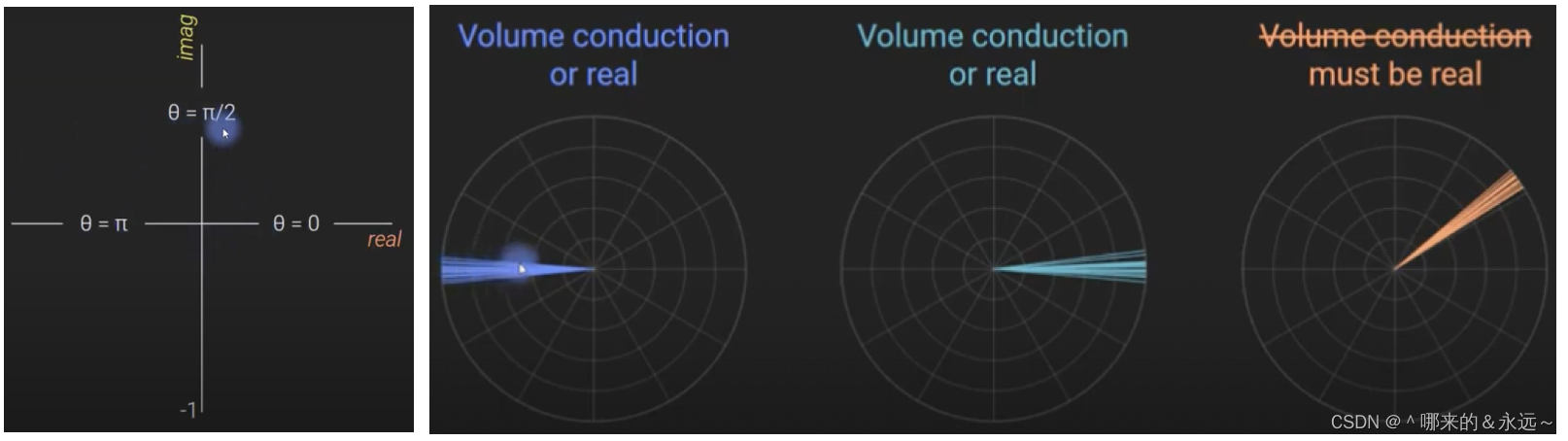
可将图中矢量视为两个电极之间的相位差。随着时间推移，会发现这些矢量沿实轴聚集。在大脑中，既存在真实的 $0$ 相位滞后同步，也存在极短时间的低延迟非 $0$ 同步。由于少量噪声和采样变异性可能使虚假同步与真实信号难以区分，因此类似前两个图中矢量沿实轴聚集的情况，既可能是体积传导导致的虚假同步，也可能是真实同步。

将前两个图与第三个图对比，第三个图中相位角的分布偏离实轴，这种分布不可能是由体积连接产生的假象。因为体积传导引发的同步具有特定的实轴分布特征，而第三个图的分布形态表明两个电极之间存在真实的相互作用，即电极实际测量的是两个神经群体之间的活动，对应真实的连通性，可避免体积传导伪影的干扰。这一现象也反映出在相位滞后测量与相位聚类测量的选择上，需权衡对体积传导的灵敏性和分析结果的稳健性。

四、PLI 的计算

PLI 计算涉及的参数定义如下：

• $n=$ 1. Number of trial/phase differences；2. Number of timePoint
  1. 试验/相位差异的数量；2. 时间点的数量

• $j=$ Phase at sensor j
  传感器 $j$ 处的相位

• $k=$ phase at sensor k
  传感器 $k$ 处的相位

• $t=$ 1. Trial; 2. timePoint
  1. 试验（编号）；2. 时间点（编号）

  

  PLI 的计算公式如下：
  $$PLI=\left|n^{-1}\sum _{t=1}^{n}sgn\left(Im\left[e^{i({\varphi }^j-{\varphi }^k)t}\right]\right)\right|$$

4.1 公式各部分含义解析

1. ${\varphi }^j-{\varphi }^k$：表示电极 $j$ 和电极 $k$ 之间的相位角差异（即相位差）。
2. $e^{i({\varphi }^j-{\varphi }^k)t}$：将上述相位差转化为复平面上的单位向量，该向量在复平面中的相位角由两个电极之间的相位差决定。
3. $Im\left[e^{i({\varphi }^j-{\varphi }^k)t}\right]$：不对相位差本身定义的角度向量进行直接处理，而是将该向量投影到虚轴上，仅考虑“相位差”向量的虚部，其值等于 $\sin ({\varphi }^j-{\varphi }^k)$。
4. $sgn\left(Im\left[e^{i({\varphi }^j-{\varphi }^k)t}\right]\right)$：符号函数（sign 函数）的作用的是：若相位差向量的虚部为负（无论负值大小），经过符号函数处理后结果为 $-1$；若虚部为正（无论正值大小），处理后结果为 $1$。

4.2 计算实例说明

• 若 $n$ 表示试验次数，例如 $n=20$，20 个试验对应的相位差向量经取虚部和符号函数处理后，结果均为 $-1$，求和后得到 $-20$。这一结果表明在当前时刻（timePoint），这 20 个试验的相位差在复平面上的投影均指向虚轴的负侧。
• 若 $n$ 表示时间点数量，例如 $n=20$，20 个时间点对应的相位差向量经取虚部和符号函数处理后，结果均为 $-1$，求和后得到 $-20$。这基本表明在当前时间段（timePeriod）内，这 20 个时刻的相位差在复平面上的投影均指向虚轴的负侧。

4.3 最终 PLI 值计算

对符号函数处理后的结果求和（即 ${\sum }_{t=1}^{n}sgn\left(Im\left[e^{i({\varphi }^j-{\varphi }^k)t}\right]\right)$），再除以 $n$ 取平均值，最后对结果取绝对值（即 $\left|n^{-1}{\sum }_{t=1}^{n}sgn\left(Im\left[e^{i({\varphi }^j-{\varphi }^k)t}\right]\right)\right|$），得到 PLI 值。

以 $n=20$ 且符号函数处理结果均为 $-1$ 为例，计算可得 $PLI=1$，这表明电极 $j$ 和电极 $k$ 之间，电极 $j$ 始终滞后于电极 $k$（或反之，需结合具体相位差定义判断），即两个电极始终保持同步，且同步程度极强。

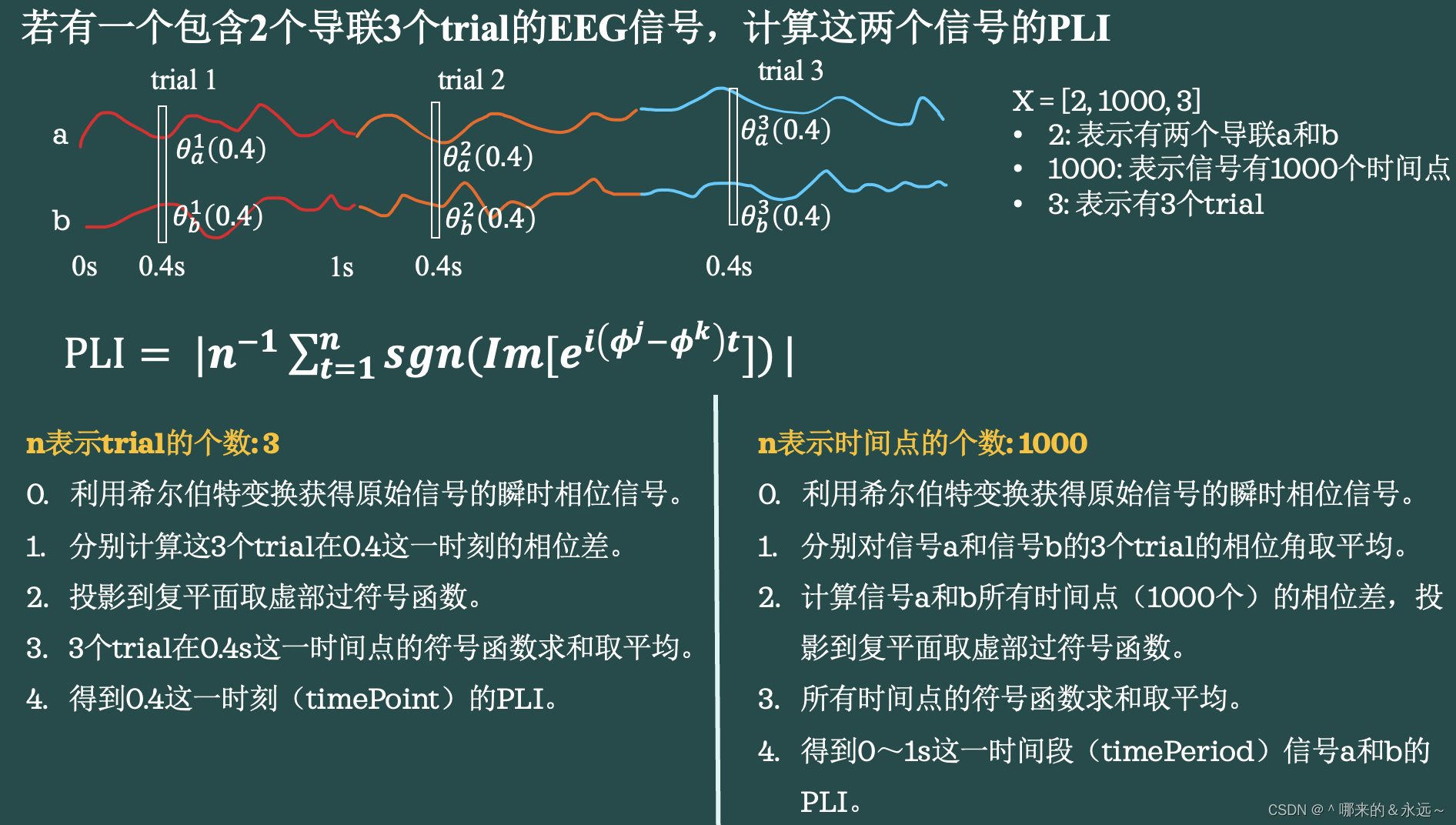
4.4 具体数据计算示例（以包含 2 个导联、3 个试验的 EEG 信号为例）

此处 PLI 计算公式表述形式：
$$PLI=\left|\frac{1}{n}\sum _{t=1}^n\text{sgn}\left(\text{Im}\left[e^{i({\varphi }^j(t)-{\varphi }^k(t))}\right]\right)\right|$$

已知 EEG 信号参数：2 个导联（分别记为 $a$ 和 $b$）、1000 个时间点、3 个试验（trial1、trial2、trial3），时间范围涉及 0s、0.4s、1s 等关键节点（具体时间点分布需结合实际数据），信号矩阵可表示为 $X=[2,1000,3]$，其中各数字分别对应导联数、时间点数、试验数。

4.4.1 当 $n$ 表示试验个数（$n=3$）时

1. 利用希尔伯特变换（Hilbert transform）获取原始信号的瞬时相位信号。
2. 分别计算 3 个试验在 0.4s 这一时刻的相位差（即导联 $a$ 与导联 $b$ 在该时刻的相位差值）。
3. 将各试验的相位差投影到复平面，取虚部后通过符号函数处理。
4. 对 3 个试验在 0.4s 这一时间点经符号函数处理后的结果求和，并取平均值，最终得到 0.4s 这一时刻（timePoint）的 PLI 值。

4.4.2 当 $n$ 表示时间点个数（$n=1000$）时

1. 利用希尔伯特变换获取原始信号的瞬时相位信号。
2. 分别对信号 $a$ 和信号 $b$ 的 3 个试验的相位角取平均，得到两个导联的平均相位角序列。
3. 计算信号 $a$ 和信号 $b$ 在所有 1000 个时间点的相位差，将各相位差投影到复平面，取虚部后通过符号函数处理。
4. 对所有时间点经符号函数处理后的结果求和，并取平均值，得到 0~1s 这一时间段（timePeriod）内信号 $a$ 和信号 $b$ 的 PLI 值。

在复平面相关计算中，需明确：$e^{i\varphi }=\cos \varphi +i\sin \varphi$，其中 $Im\left[e^{i\varphi }\right]=\sin \varphi$，$Re\left[e^{i\varphi }\right]=\cos \varphi$（$Re$ 表示实部，$Im$ 表示虚部），这是相位差投影计算的基本数学依据。

五、MATLAB 实现 PLI

function PLI = PhaseLagIndex(X, trialTimePoint, timePeriod)
    %% 输入多变量数据，返回相位滞后指数矩阵
    % trialTimePoint 和 timePeriod 用于确定计算哪种类型的 PLI
    % trialTimePoint 和 timePeriod 不能同时为 1，若同时为 0，则默认选择 timePeriod 模式
    % 基于“相位同步”相关代码修改
    % X：数据维度为 通道数 * 时间点数 * 试验数
    
    if trialTimePoint == 1 && timePeriod == 1
        trialTimePoint = 0;
    end
    if trialTimePoint == 0 && timePeriod == 0
        timePeriod = 1;
    end
    
    numChannels = size(X, 1);   % 通道数
    numTimePoint = size(X, 2);  % 时间点数
    numTrials = size(X, 3);     % 试验数
    
    %% 通过希尔伯特变换获取每个通道的瞬时相位
    dataP = zeros(size(X));
    for channelCount = 1:numChannels
        dataP(channelCount, :, :) = angle(hilbert(squeeze(X(channelCount, :, :))));
    end
    
    % 情况 1：计算某一时刻不同试验的相位差投影是否始终指向复平面同一侧
    if trialTimePoint == 1
        %% PLI 计算
        PLI = ones(numTimePoint, numChannels, numChannels);
        for ch1 = 1:numChannels - 1
            for ch2 = ch1 + 1:numChannels
                % 计算每个时间点的相位差
                PDiff = squeeze(dataP(ch1, :, :)) - squeeze(dataP(ch2, :, :));
                % 计算 PLI（仅考虑相位差的不对称性）
                PLI(:, ch1, ch2) = abs(sum(sign(sin(PDiff)), 2) / numTrials);
                PLI(:, ch2, ch1) = PLI(:, ch1, ch2);  % PLI 具有对称性
            end
        end
    end
    
    % 情况 2：计算某一时间段内相位差投影是否始终指向复平面同一侧（虚轴正侧或负侧）
    if timePeriod == 1
        % 对不同试验的相位进行平均
        phi1 = mean(dataP, 3);
        ch = numChannels;
        
        %% PLI 计算
        PLI = ones(ch, ch);
        for ch1 = 1:ch - 1
            for ch2 = ch1 + 1:ch
                % 计算相位差
                PDiff = phi1(ch1, :) - phi1(ch2, :);
                % 计算 PLI（仅考虑相位差的不对称性）
                PLI(ch1, ch2) = abs(mean(sign(sin(PDiff))));
                PLI(ch2, ch1) = PLI(ch1, ch2);  % PLI 具有对称性
            end
        end
    end
end

PLI 值的意义可通过具体数值体现：

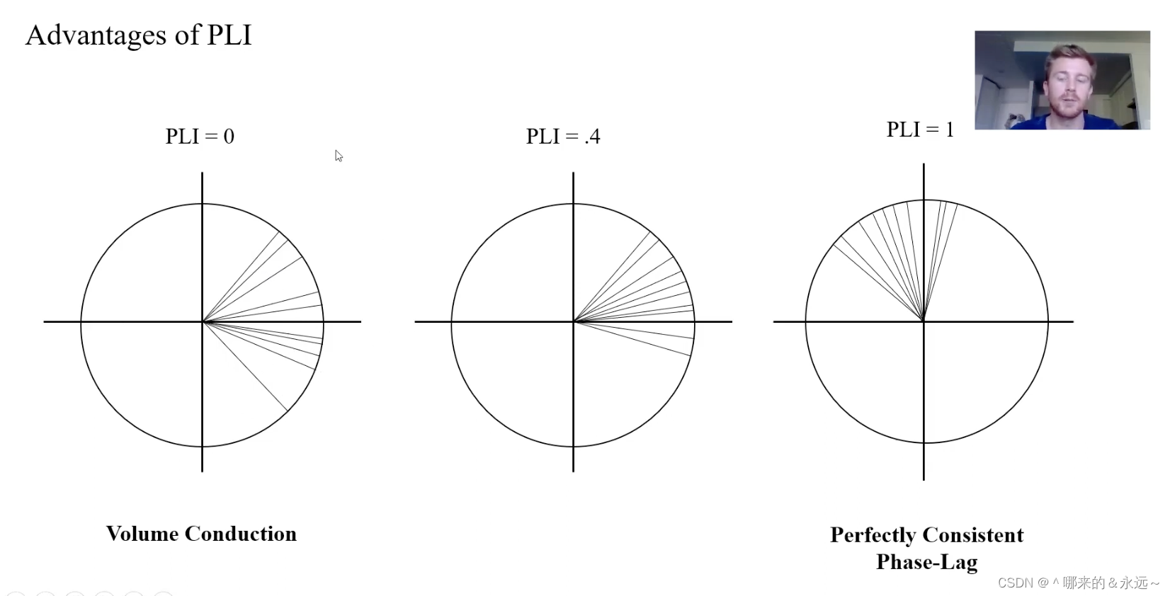
例如

• $PLI=0$ 可能对应体积传导干扰或无同步，
• $PLI=0.4$ 表示中等程度同步，
• $PLI=1$ 表示完全一致的相位滞后（完美同步）。

六、计算结果差异

采用上述两种不同 $n$ 定义（试验数或时间点数）计算某一时间区间的 PLI 时，结果可能存在显著差异。我不晓得哪个才是对的，但我更倾向于选择第一个， $n$ 表示 trial (试验个数)的计算方式。

当 $n$ 表示试验个数时，计算某一区间的 PLI 需遵循以下步骤：先计算该区间内每一个时刻的 PLI，得到所有时刻的 PLI 序列后，再对所需时间区间内的 PLI 值取平均，最终得到该区间的 PLI 结果。

七、加权相位滞后指数（wPLI, weighted Phase - Lag Index）

7.1 改进背景与基本目标

尽管 PLI 已对零滞后交互不敏感，但加权相位滞后指数（wPLI）进一步解决了由体积传导（volume conduction）引起的潜在混杂因素，提升了功能连接分析的准确性。

7.1.1 体积传导问题

体积传导是指脑电信号在头皮上传播过程中，由于脑组织和头皮的电导率存在差异，导致信号在不同电极之间传播时出现空间扩散的现象。这种扩散会使原本不相关的电极检测到虚假的信号同步性，严重干扰功能连接分析结果的可靠性，是脑电信号分析中的重要干扰因素。

7.1.2 加权机制

wPLI 通过根据相位差与实轴的距离，对相位差的贡献进行加权处理，进一步优化了 PLI 的性能。具体而言，它针对那些接近零滞后（“almost - zero - lag”）的交互进行调整，降低此类交互对最终结果的干扰。

7.1.3 “almost - zero - lag”交互

“almost - zero - lag”交互指相位差非常接近零但并非完全零滞后的情况。在实际分析中，这些交互常被视为噪声，因为它们可能掩盖真实的零滞后交互（或其他有意义的非零滞后交互）。通过加权机制，wPLI 可降低这些噪声交互的贡献权重，从而更准确地反映脑区之间真实的信号同步性。

7.2 wPLI 计算公式

$$wPLI=\frac{n^{-1}{\sum }_{t=1}^n\left|Im\left[e^{i({\theta }^j-{\theta }^k)t}\right]\right|sgn\left(Im\left[e^{i({\theta }^j-{\theta }^k)t}\right]\right)}{n^{-1}{\sum }_{t=1}^n\left|Im\left[e^{i({\theta }^j-{\theta }^k)t}\right]\right|}=\frac{{\sum }_{t=1}^{n}Im\left[e^{i({\theta }^j-{\theta }^k)t}\right]}{{\sum }_{t=1}^n\left|Im\left[e^{i({\theta }^j-{\theta }^k)t}\right]\right|}$$

公式解释

令 ${\theta }^j-{\theta }^k=\phi$，则：
$$\left|Im\left[e^{i({\theta }^j-{\theta }^k)t}\right]\right|=\left|Im\left[e^{i\phi t}\right]\right|=|\sin \phi |$$

通过分析 $|\sin \phi |$ 的变化规律，可得出以下结论：

1. 当相位差 $\phi$ 在 $0^{\circ }\sim 90^{\circ }$ 或 $180^{\circ }\sim 270^{\circ }$ 范围内时，相位差越大，$|\sin \phi |$ 值越大（即权重越大），此时相位差远离实轴，对应的交互越远离零滞后，更可能代表真实同步。
2. 当相位差 $\phi$ 在 $90^{\circ }\sim 180^{\circ }$ 或 $270^{\circ }\sim 360^{\circ }$ 范围内时，相位差越大，$|\sin \phi |$ 值越小（即权重越小），此时相位差接近实轴，对应的交互越接近零滞后，更可能是体积传导引发的噪声。

wPLI 计算的其他部分（如符号函数处理、求和与平均逻辑）与 PLI 一致，具体可参考前文 PLI 相关讲解。

八、Python 代码实现：某段时间内两个信号的 wPLI

import numpy as np
from scipy.signal import hilbert

def calculate_wPLI(signal1, signal2):
    """
    计算两个信号之间的去偏加权相位滞后指数（dwPLI）
    
    参数：
        signal1, signal2: 一维数组，形状为 (n_timepoints,)
    
    返回：
        wPLI: 标量，取值范围 [-1, 1]
        · wPLI ≈ 1：信号1始终领先信号2。
		· wPLI ≈ -1：信号1始终滞后信号2。
		· wPLI ≈ 0：无稳定相位关系。
    """
    # 1. 计算希尔伯特变换，获取解析信号
    analytic_signal1 = hilbert(signal1)
    analytic_signal2 = hilbert(signal2)
    
    # 2. 提取瞬时相位（单位：弧度）
    phase1 = np.angle(analytic_signal1)
    phase2 = np.angle(analytic_signal2)
    
    # 3. 计算相位差的正弦值（虚部）
    phase_diff = phase1 - phase2
    imag_part = np.sin(phase_diff)  # 等价于 np.imag(np.exp(1j * phase_diff))
    
    # 4. 计算加权分子和分母
    numerator = np.mean(np.abs(imag_part) * np.sign(imag_part))
    denominator = np.mean(np.abs(imag_part))
    
    # 5. 计算加权相位滞后指数（wPLI）
    wPLI = numerator / denominator
    return wPLI

示例数据

假设两信号相位差（弧度）的虚部为以下 5 个观测值：

观测点	相位差虚部 $\text{Im}(X)$
1	0.3
2	-0.2
3	0.5
4	-0.1
5	0.4

步骤 1：计算 WPLI

1.1 计算分子：$\mathbb{E}[\text{Im}(X)]$（虚部的均值）

$$\text{均值}=\frac{0.3+(-0.2)+0.5+(-0.1)+0.4}{5}=\frac{0.9}{5}=0.18$$

取绝对值：$$|0.18|=0.18$$

1.2 计算分母：$\mathbb{E}[|\text{Im}(X)|]$（虚部绝对值的均值）

$$\text{绝对值均值}=\frac{0.3+0.2+0.5+0.1+0.4}{5}=\frac{1.5}{5}=0.3$$

1.3 计算 WPLI 值

$$\text{WPLI}=\frac{0.18}{0.3}=0.6$$

---

via：

• Comparing PLI, wPLI, and dPLI — MNE-Connectivity 0.8.0.dev101+g0a32fa549 documentation
  https://mne.tools/mne-connectivity/dev/auto_examples/dpli_wpli_pli.html

• 功能连接常用的测量指标_相位滞后指数-优快云博客
  https://blog.youkuaiyun.com/u011661076/article/details/123637056

• 从公式详解相位滞后指数（Phase-Lag Index, PLI）、加权相位滞后指数 wPLI-优快云博客
  https://blog.youkuaiyun.com/qq_45538220/article/details/129873029

• EEG Functional Connectivity Analysis for the Study of the Brain Maturation in the First Year of Life 2024
  https://pdfs.semanticscholar.org/2150/feccf33494371e36e6b784e70b4d4116a8c5.pdf