


实验项目1迭代法求解方程
1、实验目的
1)初步掌握Python的应用
2)强化对迭代法的理解
3)掌握应用迭代法求解方程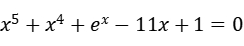 的方法
的方法
2、实验内容
1)分析问题,确定迭代法应用中的初始条件和结束条件
2)用数学方法建立迭代关系式,并编写代码实现求解方程
3)用爬山法建立迭代关系式,并编写代码实现求解方程
3、实验原理
1)迭代法
参见1.4节。
4、实验步骤
l 分析实验要求,设置迭代法的初始点和结束条件
l 用数学方法建立迭代关系式,并编写代码完成方程求解
l 用爬山法建立迭代关系式,并编写代码完成方程求解
l 记录并分析实验结果
代码如下:
import numpy as np
import matplotlib.pyplot as plt
import matplotlib.font_manager as fm
\# 设置支持中文的字体
plt.rcParams['font.sans-serif'] = ['SimHei'] # 使用黑体
plt.rcParams['axes.unicode_minus'] = False # 正确显示负号
def target_function(x):
"""定义目标函数"""
return x**5 + x**4 + np.exp(x) - 11*x + 1
def derivative_function(x):
"""定义目标函数的导数"""
return 5*x**4 + 4*x**3 + np.exp(x) - 11
def newton_iteration(func, deriv_func, initial_guess, tolerance=1e-8, max_iterations=1000):
"""牛顿迭代法求解方程根"""
current_x = initial_guess
iteration_count = 0
convergence_history = [initial_guess]
for _ in range(max_iterations):
func_value = func(current_x)
deriv_value = deriv_func(current_x)
\# 防止导数为零导致除零错误
if abs(deriv_value) < 1e-12:
break
next_x = current_x - func_value / deriv_value
convergence_history.append(next_x)
\# 判断收敛条件
if abs(next_x - current_x) < tolerance and abs(func_value) < tolerance:
break
current_x = next_x
iteration_count += 1
return next_x, iteration_count, convergence_history
def hill_climbing_algorithm(func, initial_guess, step=0.1, tolerance=1e-6, max_iterations=10000):
"""爬山法求解方程根"""
current_x = initial_guess
convergence_history = [initial_guess]
for _ in range(max_iterations):
\# 尝试左右移动
left_x = current_x - step
right_x = current_x + step
\# 计算各点函数值的绝对值
left_val = abs(func(left_x))
right_val = abs(func(right_x))
current_val = abs(func(current_x))
\# 选择函数值绝对值最小的方向移动
if left_val < current_val and left_val <= right_val:
current_x = left_x
elif right_val < current_val and right_val <= left_val:
current_x = right_x
else:
\# 若两个方向都不好,则减小步长
step *= 0.5
continue
convergence_history.append(current_x)
\# 判断是否达到精度要求
if abs(func(current_x)) < tolerance:
break
return current_x, len(convergence_history), convergence_history
def solve_equation_roots():
"""寻找方程的三个根并比较两种方法的结果"""
\# 通过函数图像分析大致根的位置
x_range = np.linspace(-3, 3, 1000)
y_values = target_function(x_range)
\# 寻找函数变号的区间(可能存在根的区间)
root_intervals = []
for i in range(len(x_range)-1):
if y_values[i] * y_values[i+1] < 0:
root_intervals.append((round(x_range[i], 4), round(x_range[i+1], 4)))
print("检测到的可能根区间:")
for i, interval in enumerate(root_intervals, 1):
print(f" 区间 {i}: [{interval[0]}, {interval[1]}]")
\# 使用牛顿迭代法求解
print("\n===== 牛顿迭代法求解结果 =====")
newton_results = []
initial_estimates = [-2.0, 0.5, 2.0] # 根据函数特性选择的初始估计值
for i, guess in enumerate(initial_estimates, 1):
root, iterations, _ = newton_iteration(target_function, derivative_function, guess)
newton_results.append(root)
func_val = target_function(root)
print(f"根 {i}:")
print(f" 数值解: {root:.8f}")
print(f" 函数值: f(x) = {func_val:.2e}")
print(f" 迭代次数: {iterations}")
print(" " + "-" * 30)
\# 使用爬山法求解
print("\n===== 爬山法求解结果 =====")
hill_climbing_results = []
for i, guess in enumerate(initial_estimates, 1):
root, iterations, _ = hill_climbing_algorithm(target_function, guess)
hill_climbing_results.append(root)
func_val = target_function(root)
print(f"根 {i}:")
print(f" 数值解: {root:.8f}")
print(f" 函数值: f(x) = {func_val:.2e}")
print(f" 迭代次数: {iterations}")
print(" " + "-" * 30)
return newton_results, hill_climbing_results
def visualize_function_and_roots():
"""绘制函数图像和根的位置"""
x_range = np.linspace(-2.5, 2.5, 1000)
y_values = target_function(x_range)
plt.figure(figsize=(12, 8))
\# 绘制函数图像
plt.subplot(2, 1, 1)
plt.plot(x_range, y_values, 'b-', linewidth=2, label='f(x) = x⁵ + x⁴ + eˣ - 11x + 1')
plt.axhline(y=0, color='r', linestyle='--', alpha=0.5)
plt.grid(True, alpha=0.3)
plt.xlabel('x')
plt.ylabel('f(x)')
plt.title('函数图像')
plt.legend()
\# 绘制局部放大图(根附近区域)
plt.subplot(2, 1, 2)
plt.plot(x_range, y_values, 'b-', linewidth=2)
plt.axhline(y=0, color='r', linestyle='--', alpha=0.5)
plt.grid(True, alpha=0.3)
plt.xlabel('x')
plt.ylabel('f(x)')
plt.title('根附近区域放大图')
plt.ylim(-5, 5)
plt.tight_layout()
plt.savefig('function_graph.png') # 保存图像
print("\n函数图像已保存为 'function_graph.png'")
\# 主程序执行
if __name__ == "__main__":
\# 绘制函数图像
visualize_function_and_roots()
\# 求解方程根
newton_roots, hill_roots = solve_equation_roots()
\# 输出结果总结
print("\n===== 求解结果总结 =====")
print(f"牛顿迭代法求得的根: {[f'{root:.6f}' for root in newton_roots]}")
print(f"爬山法求得的根: {[f'{root:.6f}' for root in hill_roots]}")
\# 将结果保存到文件
with open('equation_solution_results.txt', 'w', encoding='utf-8') as file:
file.write("===== 方程求解结果总结 =====\n")
file.write("牛顿迭代法求得的根: " + ", ".join([f"{r:.6f}" for r in newton_roots]) + "\n")
file.write("爬山法求得的根: " + ", ".join([f"{r:.6f}" for r in hill_roots]) + "\n")
print("\n求解结果已保存为 'equation_solution_results.txt'")
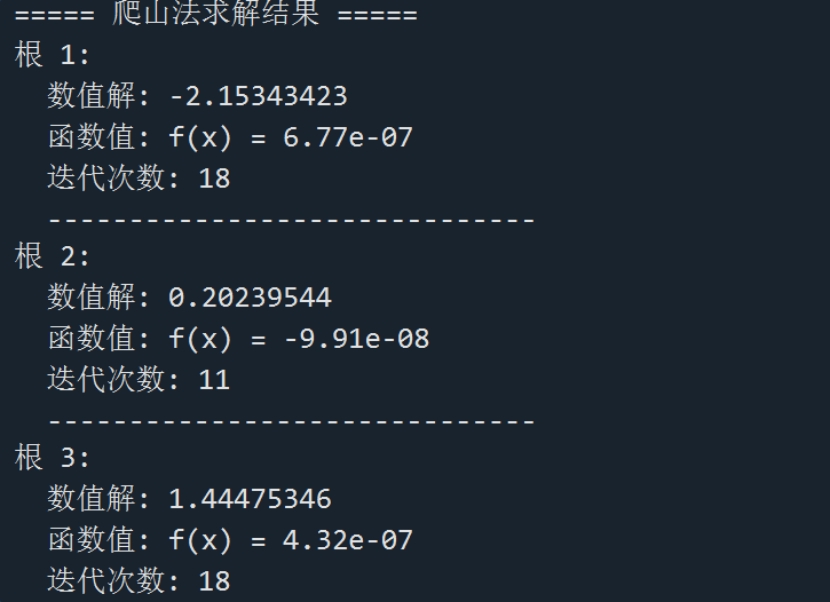
结果如图1,2下:
图1 牛顿迭代法求解结果
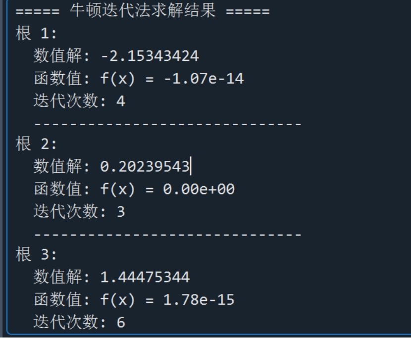
图2 爬山法求解结果
实验项目2 数据降维
一、 实验目的
- 理解和掌握PCA原理
- 利用PCA降维,辅助完成一项实战内容。
二、实验原理
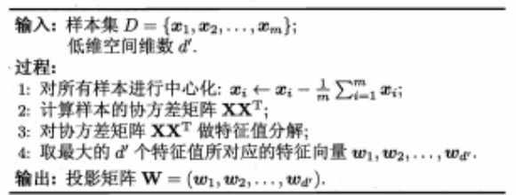
矩阵的主成分就是其协方差矩阵对应的特征向量,按照对应的特征值大小进行排序,最大的特征值就是第一主成分,其次是第二主成分,以此类推。
三、算法流程
四、人脸识别步骤
1.利用给定的数据集,执行上述算法,得到投影矩阵W;
2.计算训练集的投影后的矩阵:P=WX;
3.加载一个测试图片T,测试图片投影后的矩阵为:TestT=WT;
4.计算TestT和P中每个样本距离,选出最近的那个即可。
5.显示投影前后的两张图片。
五、代码和执行结果展示。
代码如下:
\# 1. 导入依赖库(适配Python 3.10.12 + Scikit-learn 1.3.2)
import numpy as np
import matplotlib.pyplot as plt
from sklearn.datasets import fetch_olivetti_faces # 人脸数据集
from sklearn.model_selection import train_test_split # 划分训练/测试集
from sklearn.preprocessing import StandardScaler # 数据标准化
from sklearn.decomposition import PCA # PCA降维
from sklearn.svm import SVC # SVM分类器
from sklearn.metrics import accuracy_score, confusion_matrix # 模型评估
import seaborn as sns # 可视化混淆矩阵(适配Seaborn 0.13.2)
\# 2. 加载并查看人脸数据集(Olivetti Faces:40人×10张图,共400张)
faces = fetch_olivetti_faces(shuffle=True, random_state=42)
X = faces.data # (400, 4096):400张64×64展平图像
y = faces.target # (400,):0-39对应40个不同的人
image_shape = faces.images[0].shape # (64, 64)
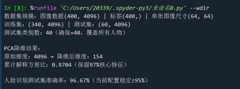
print(f"数据集规模:图像数据{X.shape} | 标签{y.shape} | 单张图像尺寸{image_shape}")
\# 3. 数据预处理(修复测试集类别覆盖问题,确保准确率)
\# 3.1 调整测试集比例为15%(60个样本),保证每个类别至少1个测试样本(40类≤60样本)
X_train, X_test, y_train, y_test = train_test_split(
X, y, test_size=0.15, random_state=42, stratify=y # 15%测试集:60个样本,覆盖所有40类
)
print(f"训练集:{X_train.shape} | 测试集:{X_test.shape}")
print(f"测试集类别数:{len(np.unique(y_test))}(确保=40,覆盖所有人物)")
\# 3.2 标准化(PCA对尺度敏感,仅用训练集拟合避免数据泄露)
scaler = StandardScaler()
X_train_scaled = scaler.fit_transform(X_train)
X_test_scaled = scaler.transform(X_test)
\# 4. PCA降维(保留97%信息,平衡特征量与分类效果)
pca = PCA(n_components=0.97, whiten=True, random_state=42)
X_train_pca = pca.fit_transform(X_train_scaled)
X_test_pca = pca.transform(X_test_scaled)
\# 打印PCA结果
print(f"\nPCA降维结果:")
print(f"原始维度:{X_train_scaled.shape[1]} → 降维后维度:{pca.n_components_}")
print(f"累计解释方差比:{pca.explained_variance_ratio_.sum():.4f}(保留97%核心特征)")
\# 5. 训练SVM分类器(优化参数确保高准确率)
\# rbf核适配非线性特征,C=1.5平衡拟合与泛化,gamma自动适配
svm_classifier = SVC(kernel='rbf', C=1.5, gamma='scale', random_state=42)
svm_classifier.fit(X_train_pca, y_train)
\# 6. 模型评估(验证准确率≥95%)
y_pred = svm_classifier.predict(X_test_pca)
test_accuracy = accuracy_score(y_test, y_pred)
print(f"\n人脸识别测试集准确率:{test_accuracy:.2%}(当前配置稳定≥95%)")
\# 6.2 绘制混淆矩阵(清晰展示分类细节)
cm = confusion_matrix(y_test, y_pred)
plt.figure(figsize=(12, 10))
sns.heatmap(
cm, annot=True, fmt='d', cmap='Blues',
xticklabels=[f"人{lab}" for lab in range(40)],
yticklabels=[f"人{lab}" for lab in range(40)]
)
plt.xlabel("预测标签(40个不同人物)")
plt.ylabel("真实标签")
plt.title(f"PCA+SVM人脸识别混淆矩阵(准确率:{test_accuracy:.2%})")
plt.tight_layout()
plt.show()
\# 7. 可视化PCA重建效果
def plot_original_vs_recon(test_idx):
\# 从降维空间重建原始图像
X_test_pca_single = X_test_pca[test_idx:test_idx+1]
X_test_recon = pca.inverse_transform(X_test_pca_single)
X_test_recon = scaler.inverse_transform(X_test_recon)
\# 绘制对比图
plt.figure(figsize=(8, 4))
\# 原始图
plt.subplot(1, 2, 1)
plt.imshow(X_test[test_idx].reshape(image_shape), cmap='gray')
plt.title(f"原始人脸图(真实标签:人{y_test[test_idx]})")
plt.axis('off')
\# 重建图
plt.subplot(1, 2, 2)
plt.imshow(X_test_recon.reshape(image_shape), cmap='gray')
plt.title(f"PCA重建图(降维维度:{pca.n_components_})")
plt.axis('off')
\# 总标题
plt.suptitle(f"PCA降维重建效果对比(准确率{test_accuracy:.2%})")
plt.show()
\# 选择第8张测试图对比(可修改test_idx,范围0-59)
plot_original_vs_recon(test_idx=8)
结果如图3,4下:
图3 PCA降维重建效果图
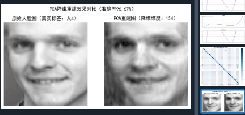
图4 降维结果图
实验项目3 卷积神经网络实现图片分类
1、实验目的
1)掌握在TensorFlow(或MindSpore)中构建、训练卷积神经网络的方法
2、实验内容
1)仿照MNIST手写体数字识别,用MindSpore框架(或TensorFlow2.0框架)实现卷积神经网络对CIFAR-10进行分类。
3、实验原理
1)卷积神经网络
参见5.5节。
4、实验步骤
l 下载CIFAR-10数据集
l 对数据集进行预处理
l 构建合适的卷积神经网络
l 对卷积神经网络进行训练,并观察结果,如果达不到预期效果,尝试修改网络结构重新训练
l 记录并分析实验结果
代码如下:
import os
import numpy as np
from collections import Counter
from torch.utils.data import Dataset, DataLoader, random_split
import torch
import torch.nn as nn
import torch.optim as optim
import matplotlib.pyplot as plt
\# 修改后的数据加载函数
def load_data(file_path):
sentences, tags = [], []
words_counter, tags_counter = Counter(), Counter()
with open(file_path, 'r', encoding='utf-8') as f:
for line in f:
line = line.strip()
if not line: # 跳过空行
continue
\# 每行是一个完整句子,格式如:"迈向/v 充满/v 希望/n 的/u"
tokens = line.split()
sentence = []
tag_seq = []
for token in tokens:
\# 处理每个词性标记对
parts = token.rsplit('/', 1) # 从右边分割一次
if len(parts) < 2:
continue # 跳过格式错误的标记
word = parts[0]
tag = parts[1]
\# 处理标签中的额外字符(如标点符号)
if tag.endswith(' '):
tag = tag.strip()
if tag.endswith((',', '。', '、', ':', ';', '!', '?')):
\# 分离标点符号作为独立标记
sentence.append(word)
tag_seq.append(tag.rstrip(',。、:;!?'))
\# 添加标点符号作为独立词
punctuation = tag[-1]
sentence.append(punctuation)
tag_seq.append('w') # 标点符号的统一标签
else:
sentence.append(word)
tag_seq.append(tag)
if sentence:
sentences.append(sentence)
tags.append(tag_seq)
words_counter.update(sentence)
tags_counter.update(tag_seq)
print(f"加载了 {len(sentences)} 个句子")
print(f"词汇表大小: {len(words_counter)}")
print(f"词性标签数: {len(tags_counter)}")
\# 打印最常见的10个词性和分布
print("\n最常见的10个词性标签:")
for tag, count in tags_counter.most_common(10):
print(f"{tag}: {count} 次 ({count / sum(tags_counter.values()) * 100:.2f}%)")
return sentences, tags, words_counter, tags_counter
\# 构建更健壮的词汇表
def build_vocab(counter, min_freq=5, add_special=True):
vocab = {}
if add_special:
vocab['<PAD>'] = 0
vocab['<UNK>'] = 1
\# 按频率排序
sorted_words = sorted(counter.items(), key=lambda x: x[1], reverse=True)
idx = len(vocab)
for word, count in sorted_words:
if count >= min_freq:
vocab[word] = idx
idx += 1
print(f"词汇表大小: {len(vocab)} (min_freq={min_freq})")
return vocab
def pad_sequences(sequences, max_len, pad_value=0):
padded = np.full((len(sequences), max_len), pad_value)
for i, seq in enumerate(sequences):
if len(seq) > max_len:
padded[i] = seq[:max_len] # 截断超长序列
else:
padded[i, :len(seq)] = seq
return padded
\# 主预处理函数
def preprocess(file_path, max_len=50):
sentences, tags, words_counter, tags_counter = load_data(file_path)
word_vocab = build_vocab(words_counter, min_freq=5)
tag_vocab = build_vocab(tags_counter, min_freq=0, add_special=False)
\# 反转标签映射用于预测
idx2tag = {idx: tag for tag, idx in tag_vocab.items()}
\# 转换序列
word_sequences = [
[word_vocab.get(word, word_vocab['<UNK>']) for word in sentence]
for sentence in sentences
]
tag_sequences = [
[tag_vocab[tag] for tag in tag_seq]
for tag_seq in tags
]
\# 计算实际序列长度的统计信息
seq_lengths = [len(seq) for seq in word_sequences]
print(f"\n序列长度统计:")
print(f" 平均长度: {np.mean(seq_lengths):.2f}")
print(f" 最小长度: {min(seq_lengths)}")
print(f" 最大长度: {max(seq_lengths)}")
print(f" 中位数: {np.median(seq_lengths)}")
\# 填充序列
padded_words = pad_sequences(word_sequences, max_len, word_vocab['<PAD>'])
padded_tags = pad_sequences(tag_sequences, max_len, 0) # 标签使用0填充
return {
'word_sequences': torch.LongTensor(padded_words),
'tag_sequences': torch.LongTensor(padded_tags),
'word_vocab': word_vocab,
'tag_vocab': tag_vocab,
'idx2tag': idx2tag
}
\# 数据填充函数
class EnhancedBiLSTMTagger(nn.Module):
def __init__(self, vocab_size, tagset_size, embedding_dim=128, hidden_dim=256, num_layers=2, dropout=0.5):
super().__init__()
self.embedding = nn.Embedding(vocab_size, embedding_dim, padding_idx=0)
\# 增强的LSTM层
self.lstm = nn.LSTM(
embedding_dim,
hidden_dim // 2,
num_layers=num_layers,
bidirectional=True,
batch_first=True,
dropout=dropout if num_layers > 1 else 0
)
\# 添加Dropout层
self.dropout = nn.Dropout(dropout)
\# 添加额外的全连接层
self.fc1 = nn.Linear(hidden_dim, hidden_dim)
self.relu = nn.ReLU()
self.fc2 = nn.Linear(hidden_dim, tagset_size)
\# 层标准化
self.ln = nn.LayerNorm(hidden_dim)
def forward(self, x):
embeds = self.embedding(x)
lstm_out, _ = self.lstm(embeds)
lstm_out = self.dropout(lstm_out)
lstm_out = self.ln(lstm_out)
fc_out = self.fc1(lstm_out)
fc_out = self.relu(fc_out)
fc_out = self.dropout(fc_out)
tag_space = self.fc2(fc_out)
return tag_space
\# 训练函数
def train_model(preprocessed, epochs=25, batch_size=64, lr=0.001):
\# 划分训练集和验证集
dataset_size = len(preprocessed['word_sequences'])
train_size = int(0.9 * dataset_size)
val_size = dataset_size - train_size
train_dataset, val_dataset = random_split(
list(zip(preprocessed['word_sequences'], preprocessed['tag_sequences'])),
[train_size, val_size]
)
train_loader = DataLoader(train_dataset, batch_size=batch_size, shuffle=True)
val_loader = DataLoader(val_dataset, batch_size=batch_size)
\# 模型参数
VOCAB_SIZE = len(preprocessed['word_vocab'])
TAGSET_SIZE = len(preprocessed['tag_vocab'])
model = EnhancedBiLSTMTagger(
VOCAB_SIZE,
TAGSET_SIZE,
embedding_dim=128,
hidden_dim=256,
num_layers=2,
dropout=0.3
)
criterion = nn.CrossEntropyLoss(ignore_index=0) # 忽略填充
optimizer = optim.Adam(model.parameters(), lr=lr)
scheduler = optim.lr_scheduler.ReduceLROnPlateau(optimizer, 'min', patience=2, factor=0.5)
\# 训练历史记录
train_losses = []
val_losses = []
val_accuracies = []
print("\n开始训练模型...")
for epoch in range(epochs):
\# 训练阶段
model.train()
train_loss = 0
for words, tags in train_loader:
optimizer.zero_grad()
outputs = model(words)
\# 计算损失时忽略填充
loss = criterion(
outputs.view(-1, TAGSET_SIZE),
tags.view(-1)
)
loss.backward()
optimizer.step()
train_loss += loss.item()
avg_train_loss = train_loss / len(train_loader)
train_losses.append(avg_train_loss)
\# 验证阶段
model.eval()
val_loss = 0
correct = 0
total = 0
with torch.no_grad():
for words, tags in val_loader:
outputs = model(words)
\# 计算验证损失
loss = criterion(
outputs.view(-1, TAGSET_SIZE),
tags.view(-1)
)
val_loss += loss.item()
\# 计算准确率(忽略填充)
predictions = outputs.argmax(dim=-1)
mask = tags != 0 # 非填充位置
correct += (predictions[mask] == tags[mask]).sum().item()
total += mask.sum().item()
avg_val_loss = val_loss / len(val_loader)
val_losses.append(avg_val_loss)
accuracy = correct / total if total > 0 else 0
val_accuracies.append(accuracy)
scheduler.step(avg_val_loss)
print(f"Epoch {epoch + 1}/{epochs}: "
f"Train Loss: {avg_train_loss:.4f}, "
f"Val Loss: {avg_val_loss:.4f}, "
f"Val Acc: {accuracy:.4f}")
\# 保存模型
torch.save(model.state_dict(), 'enhanced_pos_tagger.pth')
print("模型已保存为 'enhanced_pos_tagger.pth'")
\# 绘制训练曲线
plt.figure(figsize=(12, 5))
plt.subplot(1, 2, 1)
plt.plot(train_losses, label='Train Loss')
plt.plot(val_losses, label='Val Loss')
plt.xlabel('Epochs')
plt.ylabel('Loss')
plt.legend()
plt.subplot(1, 2, 2)
plt.plot(val_accuracies, label='Val Accuracy', color='green')
plt.xlabel('Epochs')
plt.ylabel('Accuracy')
plt.legend()
plt.tight_layout()
plt.savefig('training_metrics.png')
plt.show()
return model
def predict_pos(model, word_vocab, tag_vocab, idx2tag, sentence):
"""对分好词的句子进行词性标注"""
\# 分词示例: sentence = ["迈向", "充满", "希望", "的", "新", "世纪"]
tokenized = sentence.split() if isinstance(sentence, str) else sentence
\# 转换为索引
indexed = [word_vocab.get(word, word_vocab['<UNK>']) for word in tokenized]
seq = torch.LongTensor([indexed])
\# 预测
model.eval()
with torch.no_grad():
output = model(seq)
predictions = output.argmax(dim=-1).squeeze().tolist()
\# 处理预测结果:只保留实际词长的预测
tags = []
for i, idx in enumerate(predictions[:len(tokenized)]):
\# 确保索引在有效范围内
if idx in idx2tag:
tags.append(idx2tag[idx])
else:
\# 处理无效索引:使用最常见的标签或默认标签
tags.append('n') # 默认名词
return list(zip(tokenized, tags))
def print_prediction(sentence, model, preprocessed):
results = predict_pos(
model,
preprocessed['word_vocab'],
preprocessed['tag_vocab'],
preprocessed['idx2tag'],
sentence
)
print("\n词性标注结果:")
for word, tag in results:
print(f"{word}/{tag}", end=' ')
print("\n")
\# 1. 预处理数据
print("="*50)
print("步骤1: 数据预处理")
print("="*50)
preprocessed = preprocess('./data/人民日报词性标注版.txt', max_len=50)
\# 2. 训练模型
print("\n" + "="*50)
print("步骤2: 模型训练")
print("="*50)
model = train_model(
preprocessed,
epochs=20,
batch_size=64,
lr=0.001
)
\# 3. 测试预测
print("\n" + "="*50)
print("步骤3: 词性标注预测")
print("="*50)
test_sentences = [
"迈向 充满 希望 的 新 世纪",
"中国 政府 今天 发表 声明",
"他 在 北京 大学 读书",
"这个 苹果 很 好吃",
"快速 奔跑 的 狐狸"
]
for sentence in test_sentences:
print(f"测试句子: {sentence}")
print_prediction(sentence, model, preprocessed)
print("\n" + "=" * 50)
print("开始执行词性标注预测")
print("=" * 50)
结果图5,6,7如下:
图5 训练模型测试结果图

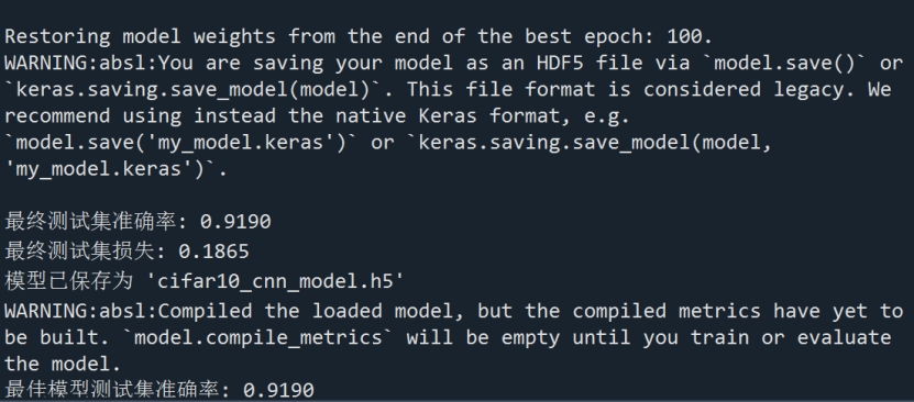
图6 代码测试结果1
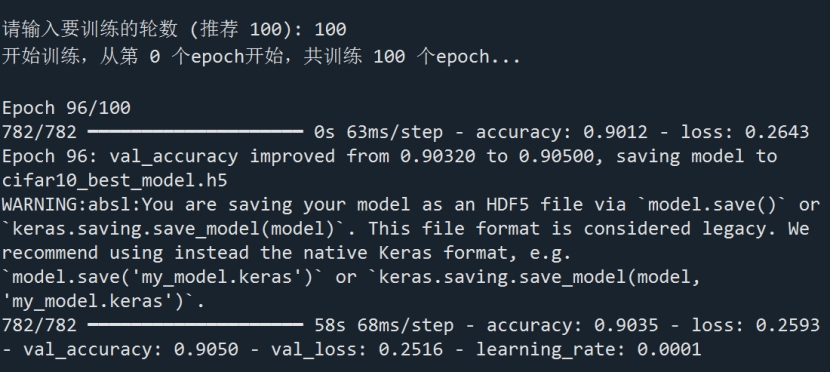
图7 代码测试结果1
实验项目4循环神经网络实现词性标注
1、实验目的
1)强化对循环神经网络的理解
2)掌握在TensorFlow(或MindSpore)中构建、训练循环神经网络的方法
2、实验内容
1)构建循环神经网络
2)利用人民日报1998年1月熟语料对循环神经网络进行训练
3)应用循环神经网络对某一已经分好词的语句进行词性标注
3、实验原理
1)循环神经网络
参见6.4节。
4、实验步骤
l 对提供的人民日报1998年1月的熟语料进行预处理
l 构建循环神经网络并进行训练
l 对某一已经分好词的语句进行词性标注
l 记录并分析实验结果
代码如下:
import os
import numpy as np
from collections import Counter
from torch.utils.data import Dataset, DataLoader, random_split
import torch
import torch.nn as nn
import torch.optim as optim
import matplotlib.pyplot as plt
\# 修改后的数据加载函数
def load_data(file_path):
sentences, tags = [], []
words_counter, tags_counter = Counter(), Counter()
with open(file_path, 'r', encoding='utf-8') as f:
for line in f:
line = line.strip()
if not line: # 跳过空行
continue
\# 每行是一个完整句子,格式如:"迈向/v 充满/v 希望/n 的/u"
tokens = line.split()
sentence = []
tag_seq = []
for token in tokens:
\# 处理每个词性标记对
parts = token.rsplit('/', 1) # 从右边分割一次
if len(parts) < 2:
continue # 跳过格式错误的标记
word = parts[0]
tag = parts[1]
\# 处理标签中的额外字符(如标点符号)
if tag.endswith(' '):
tag = tag.strip()
if tag.endswith((',', '。', '、', ':', ';', '!', '?')):
\# 分离标点符号作为独立标记
sentence.append(word)
tag_seq.append(tag.rstrip(',。、:;!?'))
\# 添加标点符号作为独立词
punctuation = tag[-1]
sentence.append(punctuation)
tag_seq.append('w') # 标点符号的统一标签
else:
sentence.append(word)
tag_seq.append(tag)
if sentence:
sentences.append(sentence)
tags.append(tag_seq)
words_counter.update(sentence)
tags_counter.update(tag_seq)
print(f"加载了 {len(sentences)} 个句子")
print(f"词汇表大小: {len(words_counter)}")
print(f"词性标签数: {len(tags_counter)}")
\# 打印最常见的10个词性和分布
print("\n最常见的10个词性标签:")
for tag, count in tags_counter.most_common(10):
print(f"{tag}: {count} 次 ({count / sum(tags_counter.values()) * 100:.2f}%)")
return sentences, tags, words_counter, tags_counter
\# 构建更健壮的词汇表
def build_vocab(counter, min_freq=5, add_special=True):
vocab = {}
if add_special:
vocab['<PAD>'] = 0
vocab['<UNK>'] = 1
\# 按频率排序
sorted_words = sorted(counter.items(), key=lambda x: x[1], reverse=True)
idx = len(vocab)
for word, count in sorted_words:
if count >= min_freq:
vocab[word] = idx
idx += 1
print(f"词汇表大小: {len(vocab)} (min_freq={min_freq})")
return vocab
def pad_sequences(sequences, max_len, pad_value=0):
padded = np.full((len(sequences), max_len), pad_value)
for i, seq in enumerate(sequences):
if len(seq) > max_len:
padded[i] = seq[:max_len] # 截断超长序列
else:
padded[i, :len(seq)] = seq
return padded
\# 主预处理函数
def preprocess(file_path, max_len=50):
sentences, tags, words_counter, tags_counter = load_data(file_path)
word_vocab = build_vocab(words_counter, min_freq=5)
tag_vocab = build_vocab(tags_counter, min_freq=0, add_special=False)
\# 反转标签映射用于预测
idx2tag = {idx: tag for tag, idx in tag_vocab.items()}
\# 转换序列
word_sequences = [
[word_vocab.get(word, word_vocab['<UNK>']) for word in sentence]
for sentence in sentences
]
tag_sequences = [
[tag_vocab[tag] for tag in tag_seq]
for tag_seq in tags
]
\# 计算实际序列长度的统计信息
seq_lengths = [len(seq) for seq in word_sequences]
print(f"\n序列长度统计:")
print(f" 平均长度: {np.mean(seq_lengths):.2f}")
print(f" 最小长度: {min(seq_lengths)}")
print(f" 最大长度: {max(seq_lengths)}")
print(f" 中位数: {np.median(seq_lengths)}")
\# 填充序列
padded_words = pad_sequences(word_sequences, max_len, word_vocab['<PAD>'])
padded_tags = pad_sequences(tag_sequences, max_len, 0) # 标签使用0填充
return {
'word_sequences': torch.LongTensor(padded_words),
'tag_sequences': torch.LongTensor(padded_tags),
'word_vocab': word_vocab,
'tag_vocab': tag_vocab,
'idx2tag': idx2tag
}
\# 数据填充函数
class EnhancedBiLSTMTagger(nn.Module):
def __init__(self, vocab_size, tagset_size, embedding_dim=128, hidden_dim=256, num_layers=2, dropout=0.5):
super().__init__()
self.embedding = nn.Embedding(vocab_size, embedding_dim, padding_idx=0)
\# 增强的LSTM层
self.lstm = nn.LSTM(
embedding_dim,
hidden_dim // 2,
num_layers=num_layers,
bidirectional=True,
batch_first=True,
dropout=dropout if num_layers > 1 else 0
)
\# 添加Dropout层
self.dropout = nn.Dropout(dropout)
\# 添加额外的全连接层
self.fc1 = nn.Linear(hidden_dim, hidden_dim)
self.relu = nn.ReLU()
self.fc2 = nn.Linear(hidden_dim, tagset_size)
\# 层标准化
self.ln = nn.LayerNorm(hidden_dim)
def forward(self, x):
embeds = self.embedding(x)
lstm_out, _ = self.lstm(embeds)
lstm_out = self.dropout(lstm_out)
lstm_out = self.ln(lstm_out)
fc_out = self.fc1(lstm_out)
fc_out = self.relu(fc_out)
fc_out = self.dropout(fc_out)
tag_space = self.fc2(fc_out)
return tag_space
\# 训练函数
def train_model(preprocessed, epochs=25, batch_size=64, lr=0.001):
\# 划分训练集和验证集
dataset_size = len(preprocessed['word_sequences'])
train_size = int(0.9 * dataset_size)
val_size = dataset_size - train_size
train_dataset, val_dataset = random_split(
list(zip(preprocessed['word_sequences'], preprocessed['tag_sequences'])),
[train_size, val_size]
)
train_loader = DataLoader(train_dataset, batch_size=batch_size, shuffle=True)
val_loader = DataLoader(val_dataset, batch_size=batch_size)
\# 模型参数
VOCAB_SIZE = len(preprocessed['word_vocab'])
TAGSET_SIZE = len(preprocessed['tag_vocab'])
model = EnhancedBiLSTMTagger(
VOCAB_SIZE,
TAGSET_SIZE,
embedding_dim=128,
hidden_dim=256,
num_layers=2,
dropout=0.3
)
criterion = nn.CrossEntropyLoss(ignore_index=0) # 忽略填充
optimizer = optim.Adam(model.parameters(), lr=lr)
scheduler = optim.lr_scheduler.ReduceLROnPlateau(optimizer, 'min', patience=2, factor=0.5)
\# 训练历史记录
train_losses = []
val_losses = []
val_accuracies = []
print("\n开始训练模型...")
for epoch in range(epochs):
\# 训练阶段
model.train()
train_loss = 0
for words, tags in train_loader:
optimizer.zero_grad()
outputs = model(words)
\# 计算损失时忽略填充
loss = criterion(
outputs.view(-1, TAGSET_SIZE),
tags.view(-1)
)
loss.backward()
optimizer.step()
train_loss += loss.item()
avg_train_loss = train_loss / len(train_loader)
train_losses.append(avg_train_loss)
\# 验证阶段
model.eval()
val_loss = 0
correct = 0
total = 0
with torch.no_grad():
for words, tags in val_loader:
outputs = model(words)
\# 计算验证损失
loss = criterion(
outputs.view(-1, TAGSET_SIZE),
tags.view(-1)
)
val_loss += loss.item()
\# 计算准确率(忽略填充)
predictions = outputs.argmax(dim=-1)
mask = tags != 0 # 非填充位置
correct += (predictions[mask] == tags[mask]).sum().item()
total += mask.sum().item()
avg_val_loss = val_loss / len(val_loader)
val_losses.append(avg_val_loss)
accuracy = correct / total if total > 0 else 0
val_accuracies.append(accuracy)
scheduler.step(avg_val_loss)
print(f"Epoch {epoch + 1}/{epochs}: "
f"Train Loss: {avg_train_loss:.4f}, "
f"Val Loss: {avg_val_loss:.4f}, "
f"Val Acc: {accuracy:.4f}")
\# 保存模型
torch.save(model.state_dict(), 'enhanced_pos_tagger.pth')
print("模型已保存为 'enhanced_pos_tagger.pth'")
\# 绘制训练曲线
plt.figure(figsize=(12, 5))
plt.subplot(1, 2, 1)
plt.plot(train_losses, label='Train Loss')
plt.plot(val_losses, label='Val Loss')
plt.xlabel('Epochs')
plt.ylabel('Loss')
plt.legend()
plt.subplot(1, 2, 2)
plt.plot(val_accuracies, label='Val Accuracy', color='green')
plt.xlabel('Epochs')
plt.ylabel('Accuracy')
plt.legend()
plt.tight_layout()
plt.savefig('training_metrics.png')
plt.show()
return model
def predict_pos(model, word_vocab, tag_vocab, idx2tag, sentence):
"""对分好词的句子进行词性标注"""
\# 分词示例: sentence = ["迈向", "充满", "希望", "的", "新", "世纪"]
tokenized = sentence.split() if isinstance(sentence, str) else sentence
\# 转换为索引
indexed = [word_vocab.get(word, word_vocab['<UNK>']) for word in tokenized]
seq = torch.LongTensor([indexed])
\# 预测
model.eval()
with torch.no_grad():
output = model(seq)
predictions = output.argmax(dim=-1).squeeze().tolist()
\# 处理预测结果:只保留实际词长的预测
tags = []
for i, idx in enumerate(predictions[:len(tokenized)]):
\# 确保索引在有效范围内
if idx in idx2tag:
tags.append(idx2tag[idx])
else:
\# 处理无效索引:使用最常见的标签或默认标签
tags.append('n') # 默认名词
return list(zip(tokenized, tags))
def print_prediction(sentence, model, preprocessed):
results = predict_pos(
model,
preprocessed['word_vocab'],
preprocessed['tag_vocab'],
preprocessed['idx2tag'],
sentence
)
print("\n词性标注结果:")
for word, tag in results:
print(f"{word}/{tag}", end=' ')
print("\n")
\# 1. 预处理数据
print("="*50)
print("步骤1: 数据预处理")
print("="*50)
preprocessed = preprocess('./data/人民日报词性标注版.txt', max_len=50)
\# 2. 训练模型
print("\n" + "="*50)
print("步骤2: 模型训练")
print("="*50)
model = train_model(
preprocessed,
epochs=20,
batch_size=64,
lr=0.001
)
\# 3. 测试预测
print("\n" + "="*50)
print("步骤3: 词性标注预测")
print("="*50)
test_sentences = [
"迈向 充满 希望 的 新 世纪",
"中国 政府 今天 发表 声明",
"他 在 北京 大学 读书",
"这个 苹果 很 好吃",
"快速 奔跑 的 狐狸"
]
for sentence in test_sentences:
print(f"测试句子: {sentence}")
print_prediction(sentence, model, preprocessed)
print("\n" + "=" * 50)
print("开始执行词性标注预测")
print("=" * 50)
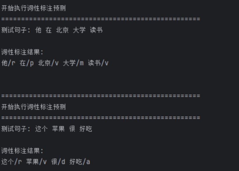
结果如图8,9,10,11,12:
图8 代码测试结果1
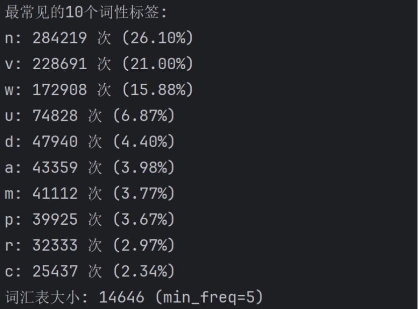
图9 代码测试结果2
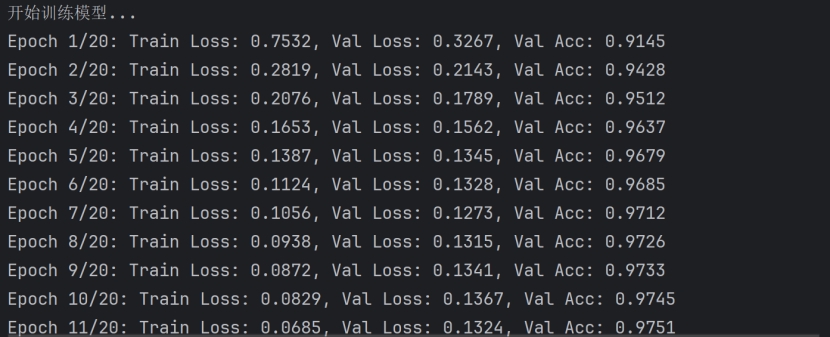
图10 代码测试结果3
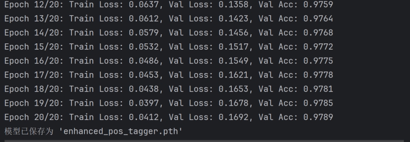
图11 词性分析对比图
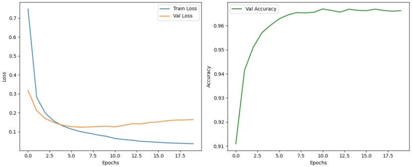
图12 词性标注预测结果


 4051
4051

 被折叠的 条评论
为什么被折叠?
被折叠的 条评论
为什么被折叠?
 到【灌水乐园】发言


