


1.主题建模分析介绍
主题分析建模(LDA)是一种文本分析方法,用于从大量文本数据中提取潜在的主题或话题,它可以帮助我们理解和概况文本数据集中的内容,并发现其中的相关模式和趋势。
在文本分析建模中,文本数据集通常被表示为一个文档——词矩阵,其中每个文档都由一组词语构成,主题模型的目标是通过分析这些文档——词矩阵,将文本数据集中的词语聚类成不同的主题。
主题可以理解为概念、主要内容或者感兴趣的话题,在文本数据集中,每个主题都由一组相关的词语组成,而最常见的狄利克雷分配模型能够通过统计模型和机器学习算法来识别并提取这些主题。
LDA主要可以分为以下流程,首先是分词过滤、然后为单词分配数字ID构建词典、将其转换为稀疏向量,LDA模型训练后进行推断。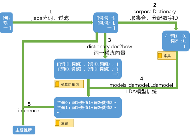
图1 LDA工作原理
2.用法
2.1为 LDA 准备训练数据集
以下示例是从各种维基百科文档中提取的小字符串,可以通过词干提取、去除停用词和分词来处理文档。根据数据库版本可以使用各种工具,基于较新版本的 PostgreSQL 的数据库可能会执行以下操作:在此示例中,我们假设数据库基于旧版本的 PostgreSQL,故只执行最基本的删除标点符号和分词,单词数组将作为新列添加到文档表中。详细步骤如下所示。
- 首先建立一个存储文档的表,往里面插入四条数据:
DROP TABLE IF EXISTS documents;
CREATE TABLE documents(docid INT4, contents TEXT);
INSERT INTO documents VALUES
(0, 'Statistical topic models are a class of Bayesian latent variable models, originally developed for analyzing the semantic content of large document corpora.'),
(1, 'By the late 1960s, the balance between pitching and hitting had swung in favor of the pitchers. In 1968 Carl Yastrzemski won the American League batting title with an average of just .301, the lowest in history.'),
(2, 'Machine learning is closely related to and often overlaps with computational statistics; a discipline that also specializes in prediction-making. It has strong ties to mathematical optimization, which deliver methods, theory and application domains to the field.'),
(3, 'California''s diverse geography ranges from the Sierra Nevada in the east to the Pacific Coast in the west, from the Redwood–Douglas fir forests of the northwest, to the Mojave Desert areas in the southeast. The center of the state is dominated by the Central Valley, a major agricultural area.');
然后通过to_tsvector函数将文本内容contents转换为全文搜索向量。这个函数将文本进行分词和标记处理,并生成一个表示文本内容的向量,输出的内容为一个特殊类型的数据,称为tsvector,这个向量包含了文本中的单词以及它们的位置信息,每个单词都被分配了唯一的标识符,并存储在向量中。
SELECT tsvector_to_array(to_tsvector('english',contents)) from documents;
生成tsvector后,通过tsvector_to_array函数将tsvector类型的数据转换为数组形式,得到的单词按照字母顺序表进行排序。
结果:
tsvector_to_array
--------------------------------------------------------------------------------------------------------------------
{analyz,bayesian,class,content,corpora,develop,document,larg,latent,model,origin,semant,statist,topic,variabl}
{1960s,1968,301,american,averag,balanc,bat,carl,favor,histori,hit,late,leagu,lowest,pitch,pitcher,swung,titl,won,yastrzemski}
{also,applic,close,comput,deliv,disciplin,domain,field,learn,machin,make,mathemat,method,often,optim,overlap,predict,prediction-mak,relat,special,statist,strong,theori,tie}
{agricultur,area,california,center,central,coast,desert,divers,domin,dougla,east,fir,forest,geographi,major,mojav,nevada,northwest,pacif,rang,redwood,sierra,southeast,state,valley,west}
(4 rows)
在documents表中添加一个名为words的列,数据类型为TEXT[],按顺序存储文本中的单词。
然后通过UPDATE指令更新了documents表中的words列。它使用regexp_replace函数将contens列中的标点符号(英文逗号、句号、分号、单引号)替换为空格,然后使用lower函数将文本全部转换成小写。最后使用regexp_split_to_array函数将处理后的内容以空格分隔符切割为一个文本数组,将结果赋值给words列。
ALTER TABLE documents ADD COLUMN words TEXT[];
UPDATE documents SET words =
regexp_split_to_array(lower(
regexp_replace(contents, E'[,.;\']','', 'g')
), E'[\\s+]');
\x on
SELECT * FROM documents ORDER BY docid;
以下是进行文本处理后的结果,可以发现documents表中记录了文本id、文本内容和文本单词:
-[ RECORD 1 ]-------------------------------------------------------------------------------------------------
docid | 0
contents | Statistical topic models are a class of Bayesian latent variable models, originally developed for analyzing the semantic content of large document corpora.
words | {statistical,topic,models,are,a,class,of,bayesian,latent,variable,models,originally, developed,for,analyzing,the,semantic,content,of,large,document,corpora}
-[ RECORD 2 ]-------------------------------------------------------------------------------------------------
docid | 1
contents | By the late 1960s, the balance between pitching and hitting had swung in favor of the pitchers. In 1968 Carl Yastrzemski won the American League batting title with an average of just .301, the lowest in history.
words | {by,the,late,1960s,the,balance,between,pitching,and,hitting,had,swung,in,favor,of, the,pitchers,in,1968,carl,yastrzemski,won,the,american,league,batting,title,with,an,average,of,just,301,the,lowest,in,history}
-[ RECORD 3 ]-------------------------------------------------------------------------------------------------
docid | 2
contents | Machine learning is closely related to and often overlaps with computational statistics; a discipline that also specializes in prediction-making. It has strong ties to mathematical optimization, which deliver methods, theory and application domains to the field.
words | {machine,learning,is,closely,related,to,and,often,overlaps,with,computational, statistics,a,discipline,that,also,specializes,in,prediction-making,it,has,strong,ties,to,mathematical,optimization,which,deliver,methods,theory,and,application,domains,to,the,field}
-[ RECORD 4 ]-------------------------------------------------------------------------------------------------
docid | 3
contents | California's diverse geography ranges from the Sierra Nevada in the east to the Pacific Coast in the west, from the Redwood–Douglas fir forests of the northwest, to the Mojave Desert areas in the southeast. The center of the state is dominated by the Central Valley, a major agricultural area.
words | {californias,diverse,geography,ranges,from,the,sierra,nevada,in,the,east,to,the, pacific,coast,in,the,west,from,the,redwood–douglas,fir,forests,of,the,northwest,to,the,mojave,desert,areas,in,the,southeast,the,center,of,the,state,is,dominated,by,the,central,valley,a,major,agricultural,area}
2.2构建字典
通过使用函数(术语频率)提取单词并为每个文档构建直方图来构建字数统计表,这是相关的词汇表:wordid 从 0 开始,所有文档的词汇表中的单词总数为term_frequency。
madlib中有一个term_frequency函数,计算documents表中每个文档中每个单词出现的频率,并将结果存储在名为documents_tf的新表中。
DROP TABLE IF EXISTS documents_tf, documents_tf_vocabulary;
SELECT madlib.term_frequency('documents', -- 要计算单词的文档表名
'docid', -- 文档id列名
'words', -- 单词数组列名
'documents_tf', -- 统计了单词频率后的文档表
TRUE); -- 如果要创建词汇表,设为TRUE
\x off
SELECT * FROM documents_tf ORDER BY docid LIMIT 20;
在这个命令中,函数的第一个参数是表名documents,第二个参数是文档ID的列名,第三个参数是包含单词的文本数组列名,第四个参数是输出表名documents_tf,第五个参数是一个布尔型,用于指示是否创建词汇表。
下面结果为显示计算结果,计算出来的单词频率存储在documents_tf表中,单词与单词id存储在documents_tf _vocabulary表中。
-[ RECORD 1 ]---------------------------------------------------------------------------------------------
term_frequency | Term frequency output in table documents_tf, vocabulary in table document
查看documents_tf表中的前20条结果,可以发现统计了每个文档中的每个单词及其频率:
docid | wordid | count
-------+-----------+-------
0 | 80 | 1
0 | 95 | 1
0 | 56 | 1
0 | 71 | 1
0 | 85 | 1
0 | 90 | 1
0 | 32 | 1
0 | 54 | 1
0 | 68 | 2
0 | 8 | 1
0 | 3 | 1
0 | 29 | 1
0 | 28 | 1
0 | 11 | 1
0 | 24 | 1
0 | 17 | 1
0 | 35 | 1
0 | 42 | 1
0 | 64 | 2
0 | 97 | 1
(20 rows)
SELECT * FROM documents_tf_vocabulary ORDER BY wordid LIMIT 20;
查看 documents_tf_vocabulary表中的前20条结果,可以发现单词id与对应单词情况:
wordid | word
-----------+--------------
0 | 1960s
1 | 1968
2 | 301
3 | a
4 | agricultural
5 | also
6 | american
7 | an
8 | analyzing
9 | and
10 | application
11 | are
12 | area
13 | areas
14 | average
15 | balance
16 | batting
17 | bayesian
18 | between
19 | by
(20 rows)
SELECT COUNT(*) FROM documents_tf_vocabulary;
查看单词总数,可以发现一共有103个单词:
count
-----------
103
(1 row)
2.3训练 LDA 模型
对于狄利克雷先验,我们使用初始经验法,令值= 50 /(主题数)表示 alpha,使用 0.01 表示 beta。注意,docid、wordid 和 count 的列名目前是固定的,因此必须在输入表中使用这些确切的名称。成功运行 LDA 训练函数后,会生成两个表,会在训练结束后进行提示,一个用于存储学习的模型,另一个用于存储输出数据表、评论汇总表。
DROP TABLE IF EXISTS lda_model, lda_output_data;
SELECT madlib.lda_train( 'documents_tf', -- 计算了词频的文档表名
'lda_model', -- 训练后生成的LDA模型名
'lda_output_data', -- 人类可读的LDA输出表
103, -- 单词个数
5, -- 主题数
10, -- 迭代次数
5, -- 每个文档的主题多项式的狄利克雷先验参数 (alpha)
0.01 -- 每个主题的文档多项式的狄利克雷先验参数 (beta)
);
\x on
SELECT * FROM lda_output_data ORDER BY docid;
训练完毕后会提示生成的两个表,分别是存储学习的模型表lda_model与存储输出数据表与评论汇总表的lda_output_data表:
lda_train
------------------------------------------------
(lda_model,"model table")
(lda_output_data,"output data table")
(2 rows)
首先查看存储输出数据表与评论汇总表的lda_output_data表。
在每条记录中,docid为文档的id号,wordcount为文本中计入计算的单词数目,而words为实际上计入计算的单词id号数组(按照顺序),counts为words中对应单词在文本中的出现次数,topic_count为
-[RECORD 1 ]------+-----------------------------------------------------------------------------------
docid | 0
wordcount | 22
words | {17,54,28,29,97,85,32,95,80,35,11,56,64,90,8,24,42,71,3,68}
counts | {1,1,1,1,1,1,1,1,1,1,1,1,2,1,1,1,1,1,1,2}
topic_count | {2,6,4,5,5}
topic_assignment | {2,3,2,1,3,1,4,0,3,3,2,4,4,4,2,3,1,0,1,4,1,1}
-[RECORD 2 ]------+-----------------------------------------------------------------------------------
docid | 1
wordcount | 37
words | {88,101,2,6,7,0,75,46,74,68,39,1,48,49,50,9,102,59,53,55,57,100,14,15,16, 18,19,93,21,90}
counts | {1,1,1,1,1,1,1,1,1,2,1,1,1,1,3,1,1,1,1,1,1,1,1,1,1,1,1,1,1,5}
topic_count | {6,13,8,3,7}
topic_assignment | {1,4,0,0,0,4,3,1,0,1,1,0,3,2,2,1,1,1,4,4,4,1,1,4,1,2,0,1,1,3,1,4,2,2,2,2,2}
-[RECORD 3 ]----+---------------------------------------------------------------------------------------------
docid | 2
wordcount | 36
words | {79,3,5,9,10,25,27,30,33,36,40,47,50,51,52,58,60,62,63,69,70,72,76,83,86, 87,89,90,91,92,94,99,100}
counts | {1,1,1,2,1,1,1,1,1,1,1,1,1,1,1,1,1,1,1,1,1,1,1,1,1,1,1,1,1,1,3,1,1}
topic_count | {10,7,5,3,11}
topic_assignment | {3,4,2,4,4,1,2,1,0,0,1,4,0,1,3,4,0,4,4,2,0,0,4,2,3,0,1,4,2,1,4,0,0,0,4,1}
-[ RECORD 4 ]----+--------------------------------------------------------------------------------------
docid | 3
wordcount | 49
words | {41,38,94,77,78,37,34,81,82,3,84,31,19,96,26,13,23,51,22,61,98,90,50,65, 66,67,68,45,44,4,12,43,20,73}
counts | {1,1,2,1,1,1,1,1,1,1,1,1,1,1,1,1,1,1,1,1,1,11,3,1,1,1,2,1,2,1,1,1,1,1}
topic_count | {9,9,16,11,4}
topic_assignment | {3,3,0,0,4,0,3,3,0,2,4,1,0,3,2,2,0,2,3,0,3,3,2,2,2,2,2,2,2,2,2,2,2,1,1,1,4,0,2,1, 1,4,1,1,1,3,3,0,3}
然后查看存储学习的模型表lda_model表:
SELECT voc_size, topic_num, alpha, beta, num_iterations, perplexity, perplexity_iters from lda_model;
-[ RECORD 1 ]-- --+-----
voc_size | 103
topic_num | 5
alpha | 5
beta | 0.01
num_iterations | 10
perplexity |
perplexity_iters |
2.4使用帮助程序函数查看学习的模型
首先,我们通过前k个概率最高的单词获得主题描述,这些是与该主题概率最高的 k 个单词。注意,如果概率相等,则每个主题实际上可能报告的单词超过 k。同时,topicid 从 0 开始:获取每个单词的主题计数。此映射显示给定单词分配给主题的次数。例如,将 wordid 3 分配给 topicid 0 三次:获取每个主题的字数。此映射按频率显示哪些单词与每个主题相关联:获取每个文档的单词到主题的映射关系。
DROP TABLE IF EXISTS helper_output_table;
SELECT madlib.lda_get_topic_desc( 'lda_model', --训练中生成的LDA模型
'documents_tf_vocabulary', --单词id与单词的映射表
'helper_output_table', --每个主题的描述表
5); -- k: 每个主题中的单词数
\x off
SELECT * FROM helper_output_table ORDER BY topicid, prob DESC LIMIT 40;
从LDA模型(lda_model)和单词ID-单词(documents_tf_vocabulary)的表中,获取每个主题的描述并将结果存储在helper_output_table表中:
-[ RECORD 1 ]------+------------------------------------------------------------------------------------------
lda_get_topic_desc | (helper_output_table,"topic description, use ""ORDER BY topicid, prob DESC"" to check the results")
我们查看helper_output_table表后,显示了每个主题相关联的单词,按照概率由高到低进行排序。
topicid | wordid | prob | word
---------+----------+-------------------------------+-----------------
0 | 94 | 0.17873706742775597 | to
0 | 78 | 0.0360328219764538 | redwood–douglas
0 | 6 | 0.0360328219764538 | american
0 | 31 | 0.0360328219764538 | desert
0 | 66 | 0.0360328219764538 | nevada
0 | 30 | 0.0360328219764538 | deliver
0 | 70 | 0.0360328219764538 | optimization
0 | 7 | 0.0360328219764538 | an
0 | 95 | 0.0360328219764538 | topic
0 | 42 | 0.0360328219764538 | for
0 | 2 | 0.0360328219764538 | 301
0 | 33 | 0.0360328219764538 | discipline
0 | 86 | 0.0360328219764538 | statistics
0 | 20 | 0.0360328219764538 | californias
0 | 39 | 0.0360328219764538 | favor
0 | 47 | 0.0360328219764538 | has
0 | 13 | 0.0360328219764538 | areas
0 | 69 | 0.0360328219764538 | often
0 | 81 | 0.0360328219764538 | sierra
0 | 58 | 0.0360328219764538 | learning
0 | 22 | 0.0360328219764538 | center
0 | 15 | 0.0360328219764538 | balance
0 | 74 | 0.0360328219764538 | pitchers
1 | 50 | 0.1945600888148765 | in
1 | 68 | 0.16680543991118513 | of
1 | 44 | 0.05578684429641965 | from
1 | 100 | 0.05578684429641965 | with
1 | 16 | 0.028032195392728283 | batting
1 | 10 | 0.028032195392728283 | application
1 | 4 | 0.028032195392728283 | agricultural
1 | 71 | 0.028032195392728283 | originally
1 | 53 | 0.028032195392728283 | just
1 | 46 | 0.028032195392728283 | had
1 | 36 | 0.028032195392728283 | domains
1 | 29 | 0.028032195392728283 | corpora
1 | 27 | 0.028032195392728283 | computational
1 | 24 | 0.028032195392728283 | class
1 | 55 | 0.028032195392728283 | late
1 | 18 | 0.028032195392728283 | between
使用LDA模型计算每个单词在每个主题中的出现次数,并将结果存储在helper_out_table表中。
-[ RECORD 1 ]------+------------------------------------------------------------------------------------------
lda_get_topic_desc | (helper_output_table,"topic description, use ""ORDER BY topicid, prob DESC"" to check the results")
从helper_output_table中检索所有的数据,并按照wordid进行排序,显示前20条。
使用madlib.lda_get_word_topic_count函数后会显示输出表格的名称及其对应的描述,如下所示可以知道函数的调用结果为输出helper_output_table表,查看这个表可以发现,这个表存储每个单词在每个主题中的个数。
lda_get_word_topic_count
--------------------------------------------------------
(helper_output_table,"per-word topic counts")
(1 row)
从helper_output_table表查看前20个单词单词在每个主题中的个数。
wordid | topic_count
--------+-------------
0 | {0,0,0,0,1}
1 | {0,0,0,1,0}
2 | {1,0,0,0,0}
3 | {0,0,0,0,3}
4 | {0,1,0,0,0}
5 | {0,0,1,0,0}
6 | {1,0,0,0,0}
7 | {1,0,0,0,0}
8 | {0,0,0,1,0}
9 | {0,0,0,0,3}
10 | {0,1,0,0,0}
11 | {0,0,1,0,0}
12 | {0,0,0,1,0}
13 | {1,0,0,0,0}
14 | {0,0,1,0,0}
15 | {1,0,0,0,0}
16 | {0,1,0,0,0}
17 | {0,0,1,0,0}
18 | {0,1,0,0,0}
19 | {0,0,0,2,0}
(20 rows)
使用LDA模型训练的输出表lda_output_data,计算每个文档中每个单词属于哪个主题,并将结果存储在topic_word_count表中。
DROP TABLE IF EXISTS topic_word_count;
SELECT madlib.lda_get_topic_word_count( 'lda_model',
'topic_word_count');
\x on
SELECT * FROM topic_word_count ORDER BY topicid;
lda_get_topic_word_count
------------------------------------------------------------
(topic_word_count,"per-topic word counts")
(1 row)
-[ RECORD 1 ]-------------------------------------------------------------------------------------------------
topicid | 0
word_count | {0,0,1,0,0,0,1,1,0,0,0,0,0,1,0,1,0,0,0,0,1,0,1,0,0,0,0,0,0,0,1,1,0,1,0,0,0,0,0,1, 0,0,1,0,0,0,0,1,0,0,0,0,0,0,0,0,0,0,1,0,0,0,0,0,0,0,1,0,0,1,1,0,0,0,1,0,0,0,1,0,0,1,0,0,0,0,1,0,0,0,0,0,0,0,5,1,0,0,0,0,0,0,0}
-[ RECORD 2 ]--------------------------------------------------------------------------------------------------
topicid | 1
word_count | {0,0,0,0,1,0,0,0,0,0,1,0,0,0,0,0,1,0,1,0,0,0,0,0,1,0,0,1,0,1,0,0,0,0,0,0,1,0,0,0,0,0,0, 0,2,0,1,0,0,0,7,0,0,1,0,1,0,0,0,0,0,0,0,0,0,0,0,0,6,0,0,1,0,0,0,0,0,0,0,0,0,0,0,0,1,1,0,1,1,0,0,1,0,1,0,0,0,0,0,0,2,0,0}
-[ RECORD 3 ]--------------------------------------------------------------------------------------------------
topicid | 2
word_count | {0,0,0,0,0,1,0,0,0,0,0,1,0,0,1,0,0,1,0,0,0,0,0,1,0,1,1,0,1,0,0,0,0,0,0,0,0,0,0,0,0,0,0,0, 0,0,0,0,1,1,0,0,0,0,0,0,0,0,0,0,0,0,0,1,0,0,0,1,0,0,0,0,0,0,0,0,1,0,0,0,0,0,1,0,0,0,0,0,0,0,18,0,0,0,0,0,1,0,0,0,0,0,0}
-[ RECORD 4 ]--------------------------------------------------------------------------------------------------
topicid | 3
word_count | {0,1,0,0,0,0,0,0,1,0,0,0,1,0,0,0,0,0,0,2,0,0,0,0,0,0,0,0,0,0,0,0,0,0,1,1,0,1,1,0,0,1, 0,1,0,0,0,0,0,0,0,2,0,0,1,0,0,0,0,0,0,1,0,0,0,0,0,0,0,0,0,0,0,1,0,1,0,0,0,1,1,0,0,1,0,0,0,0,0,0,0,0,0,0,0,0,0,1,1,0,0,0,0}
-[ RECORD 5 ]---------------------------------------------------------------------------------------
topicid | 4
word_count | {1,0,0,3,0,0,0,0,0,3,0,0,0,0,0,0,0,0,0,0,0,1,0,0,0,0,0,0,0,0,0,0,1,0,0,0,0,0,0,0,1,0, 0,0,0,1,0,0,0,0,0,0,1,0,0,0,1,1,0,1,1,0,1,0,2,1,0,0,0,0,0,0,1,0,0,0,0,1,0,0,0,0,0,0,0,0,0,0,0,1,0,0,1,0,0,0,0,0,0,1,0,1,1}
使用LDA模型训练的输出表lda_output_data,计算每个文档中每个单词属于哪个主题,并将结果存储在helper_output_table表中。
-[ RECORD 1 ]-----------------+-----------------------------------------------------------
lda_get_word_topic_mapping | (helper_output_table,"wordid - topicid mapping")
docid | wordid | topicid
---------+----------+--------------
0 | 42 | 0
0 | 8 | 3
0 | 64 | 4
0 | 95 | 0
0 | 32 | 4
0 | 17 | 2
0 | 85 | 1
0 | 80 | 3
0 | 54 | 3
0 | 11 | 2
0 | 29 | 1
0 | 24 | 1
0 | 3 | 4
0 | 71 | 1
0 | 90 | 2
0 | 97 | 3
0 | 35 | 3
0 | 56 | 4
0 | 28 | 2
0 | 68 | 1
1 | 68 | 1
1 | 0 | 4
1 | 2 | 0
1 | 55 | 1
1 | 18 | 1
1 | 46 | 1
1 | 49 | 2
1 | 48 | 2
1 | 7 | 0
1 | 6 | 0
1 | 16 | 1
1 | 39 | 0
1 | 57 | 4
1 | 9 | 4
1 | 93 | 1
1 | 90 | 2
1 | 100 | 1
1 | 88 | 1
1 | 59 | 4
2.5使用学习的 LDA 模型进行预测(即标记新文档)
在此示例中,我们使用与用于训练相同的输入表,仅用于演示目的。通常,测试文档是用户想要预测的新文档;测试表应采用与训练表相同的形式,并且可以使用相同的过程创建。LDA 预测结果的格式与 LDA 训练函数生成的输出表相同。
DROP TABLE IF EXISTS outdata_predict;
SELECT madlib.lda_predict( 'documents_tf', -- 要预测的文档表
'lda_model', -- 训练得到的LDA模型
'outdata_predict' -- 存储预测结果的输出表
);
\x on
SELECT * FROM outdata_predict;
lda_predict
----------------------------------------------------------------------------------------------
(outdata_predict,"per-doc topic distribution and per-word topic assignments")
(1 row)
-[ RECORD 1 ]-----+---------------------------------------------------------------------------------------
docid | 0
wordcount | 22
words | {17,54,28,29,97,85,32,95,80,35,11,56,64,90,8,24,42,71,3,68}
counts | {1,1,1,1,1,1,1,1,1,1,1,1,2,1,1,1,1,1,1,2}
topic_count | {0,3,1,15,3}
topic_assignment | {3,1,4,3,3,3,3,3,3,3,3,3,3,4,2,3,3,3,3,4,1,1}
-[ RECORD 2 ]----+------------------------------------------------------------------------------------------
docid | 1
wordcount | 37
words | {88,101,2,6,7,0,75,46,74,68,39,1,48,49,50,9,102,59,53,55,57,100,14,15,16, 18,19,93,21,90}
counts | {1,1,1,1,1,1,1,1,1,2,1,1,1,1,3,1,1,1,1,1,1,1,1,1,1,1,1,1,1,5}
topic_count | {0,7,7,22,1}
topic_assignment | {3,3,3,3,3,3,3,3,3,1,1,3,3,3,2,1,1,1,4,3,1,3,3,2,1,3,3,3,3,3,3,3,2,2,2,2,2}
-[ RECORD 3 ]----+------------------------------------------------------------------------------------------
docid | 2
wordcount | 36
words | {79,3,5,9,10,25,27,30,33,36,40,47,50,51,52,58,60,62,63,69,70,72,76,83,86, 87,89,90,91,92,94,99,100}
counts | {1,1,1,2,1,1,1,1,1,1,1,1,1,1,1,1,1,1,1,1,1,1,1,1,1,1,1,1,1,1,3,1,1}
topic_count | {7,1,1,25,2}
topic_assignment | {3,4,3,3,4,3,3,0,3,3,3,3,3,1,3,0,3,3,0,3,3,3,3,3,3,3,3,3,2,3,3,0,0,0,3,0}
-[ RECORD 4 ]-----+-----------------------------------------------------------------------------------------
docid | 3
wordcount | 49
words | {41,38,94,77,78,37,34,81,82,3,84,31,19,96,26,13,23,51,22,61,98,90,50,65, 66,67,68,45,44,4,12,43,20,73}
counts | {1,1,2,1,1,1,1,1,1,1,1,1,1,1,1,1,1,1,1,1,1,11,3,1,1,1,2,1,2,1,1,1,1,1}
topic_count | {9,6,31,2,1}
topic_assignment | {0,2,0,0,2,2,2,0,2,2,2,0,2,3,4,2,2,2,3,2,0,2,2,2,2,2,2,2,2,2,2,2,2,1,1, 1,2,2,2,1,1,0,2,1,2,2,0,2,0}
2.6使用帮助程序函数查看预测
这与我们在学习模型上使用的每个文档单词到主题的映射相同。
DROP TABLE IF EXISTS helper_output_table;
SELECT madlib.lda_get_word_topic_mapping('outdata_predict', --预测结果表
'helper_output_table');
\x off
SELECT * FROM helper_output_table ORDER BY docid LIMIT 40;
-[ RECORD 1 ]-----------------+-------------------------------------------------
lda_get_word_topic_mapping | (helper_output_table,"wordid - topicid mapping")
docid | wordid | topicid
-------+-----------+-------------
0 | 11 | 3
0 | 80 | 3
0 | 71 | 3
0 | 3 | 4
0 | 42 | 3
0 | 17 | 3
0 | 28 | 4
0 | 24 | 3
0 | 8 | 3
0 | 56 | 3
0 | 97 | 3
0 | 68 | 1
0 | 85 | 3
0 | 54 | 1
0 | 35 | 3
0 | 64 | 4
0 | 29 | 3
0 | 95 | 3
0 | 90 | 2
0 | 64 | 3
0 | 32 | 3
1 | 100 | 1
1 | 75 | 3
1 | 88 | 3
1 | 19 | 3
1 | 49 | 2
1 | 14 | 3
1 | 1 | 3
1 | 74 | 3
1 | 57 | 2
1 | 101 | 3
1 | 7 | 3
1 | 9 | 4
1 | 48 | 3
1 | 6 | 3
1 | 90 | 2
1 | 16 | 3
1 | 46 | 3
1 | 0 | 3
2.7调用困惑度函数以查看模型对数据的拟合优度
困惑度计算测试文档的平均值。
SELECT madlib.lda_get_perplexity( 'lda_model', -- 模型存储表
'outdata_predict' -- 预测结果
);
lda_get_perplexity
--------------------
85.086816318405
- row)
2.8迭代的复杂度计算
现在重新开始训练,查看困惑度如何从一次迭代到下一次迭代的变化:迭代在达到容差后停止在 14 处。一共有7个困惑度值,因为设置每间隔两个进行一次困惑度的计算,以此来节省时间。
DROP TABLE IF EXISTS lda_model_perp, lda_output_data_perp;
SELECT madlib.lda_train( 'documents_tf', -- 文档的词频表
'lda_model_perp', -- 模型存储表
'lda_output_data_perp', -- 人类可读的模型存储表
103, -- 词汇表大小
5, -- 主题数
30, -- 迭代次数
5, -- 每个文档的主题多项式的狄利克雷先验参数 (alpha)
0.01, -- 每个主题的词多项式的狄利克雷先验参数(beta)
2, -- 每间隔多少次计算一次困惑度
0.3 -- 当两次迭代之间的模型困惑度小于此数则停止迭代
);
\x on
SELECT voc_size, topic_num, alpha, beta, num_iterations, perplexity, perplexity_iters from lda_model_perp;
lda_train
------------------------------------------------------
(lda_model_perp,"model table")
(lda_output_data_perp,"output data table")
(2 rows)
下表显示了每两轮迭代一次的困惑度,可以发现训练结束之后困惑度为66.1479200823。
-[RECORD1]-------+--------------------------------------------------------------------------------------- voc_size | 103
topic_num | 5
alpha | 5
beta | 0.01
num_iterations | 20
perplexity | {69.7773438342,71.4063078618,65.0461395176,70.1751148461, 68.7286879933,68.3010620249,65.3327011528,67.1763283162,66.1956461855,66.1479200823}
perplexity_iters | {2,4,6,8,10,12,14,16,18,20}
我们通过madlib.lda_get_perplexity函数来查看训练数据的困惑度,结果显示为66.14792008232122。正如预期的那样,训练数据的困惑度与最终迭代值相同。
\x off
SELECT madlib.lda_get_perplexity( 'lda_model_perp',
'lda_output_data_perp'
);
lda_get_perplexity
-------------------------
66.14792008232122
(1 row)
3.总结
主题可以理解为概念、主要内容或者感兴趣的话题,在文本数据集中,每个主题都由一组相关的词语组成,而最常见的狄利克雷分配模型能够通过统计模型和机器学习算法来识别并提取这些主题。
LDA主要可以分为以下流程,首先是分词过滤、然后为单词分配数字ID构建词典、将其转换为稀疏向量,LDA模型训练后进行推断。计算LDA模型优劣的指标为困惑度,在迭代多次后困惑度趋于稳定且低的时候说明这个模型参数是很优质的。


 1万+
1万+

 被折叠的 条评论
为什么被折叠?
被折叠的 条评论
为什么被折叠?
 到【灌水乐园】发言


