Machine Learning-Ex5（吴恩达课后习题）Regularized Linear Regression and Bias v.s. Variance

目录

1. Regularized Linear Regression

1.1 Visualizing the dataset

1.2 Regularized linear regression cost function

1.3 Regularized linear regression gradient

1.4 Fitting linear regression

2. Bias-Variance

2.1 Learning curves

3. Polynomial regression

3.1 Learning Polynomial Regression

3.2 Adjusting the regularization parameter

​3.3 Selecting λ using a cross validation set 

3.4 Computing test set error

---

1. Regularized Linear Regression

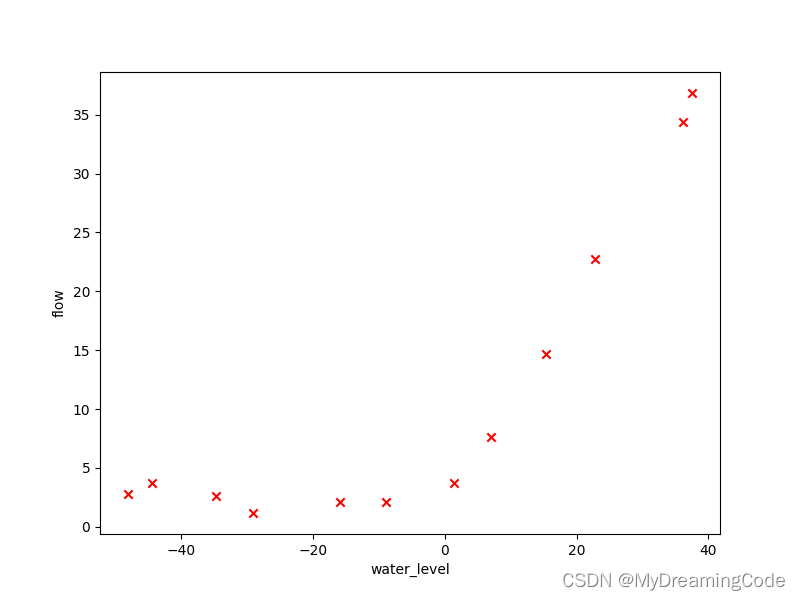
内容：我们将用正则化线性回归，使用水库中水位的变化来预测从大坝流出的水量。

1.1 Visualizing the dataset

内容：水位—X；水流量—y。将数据分成训练集、交叉验证集以及测试集。

plot.py

import matplotlib.pyplot as plt

def plotTrainingData(X, y):
    fig, ax = plt.subplots(figsize=(8, 6))
    ax.scatter(X, y, marker='x', c='r')
    ax.set_xlabel('water_level')
    ax.set_ylabel('flow')
    plt.show()

main.py

from scipy.io import loadmat  # 导入matlab格式数据
from plot import *  # 绘图

data = loadmat('ex5data.mat')
X, y, Xval, yval, Xtest, ytest = data['X'], data['y'], data['Xval'], data['yval'], data['Xtest'], data['ytest']
# print(X.shape, y.shape, Xval.shape, yval.shape, Xtest.shape, ytest.shape) #(12, 1) (12, 1) (21, 1) (21, 1) (21, 1) (21, 1)
plotTrainingData(X, y)

1.2 Regularized linear regression cost function

内容：计算带正则项的代价函数。

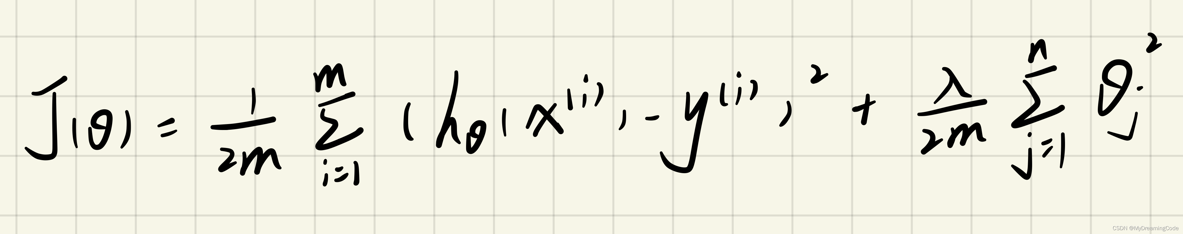
内容：正则化相当于在代价函数中增加了惩罚项，当theta(j)增大时，惩罚项也会增大。注意不需要将theta(0)进行正则化。

linearRegCostFunction.py

import numpy as np

def linearRegCostFunction(theta, X, y, learningRate):
    theta = np.matrix(theta)
    m = X.shape[0]
    X = np.insert(X, 0, np.ones(m), axis=1)
    reg = (learningRate / (2 * m)) * np.sum(np.power(theta[1:, :], 2))
    return np.sum(np.power(X * theta.T - y, 2)) / (2 * m) + reg

main.py

from scipy.io import loadmat  # 导入matlab格式数据
from linearRegCostFunction import *  # 正则化代价函数

data = loadmat('ex5data.mat')
X, y, Xval, yval, Xtest, ytest = data['X'], data['y'], data['Xval'], data['yval'], data['Xtest'], data['ytest']
theta = [1, 1]
learningRate = 1
print(linearRegCostFunction(theta, X, y, learningRate))  # 303.9515255535976

1.3 Regularized linear regression gradient

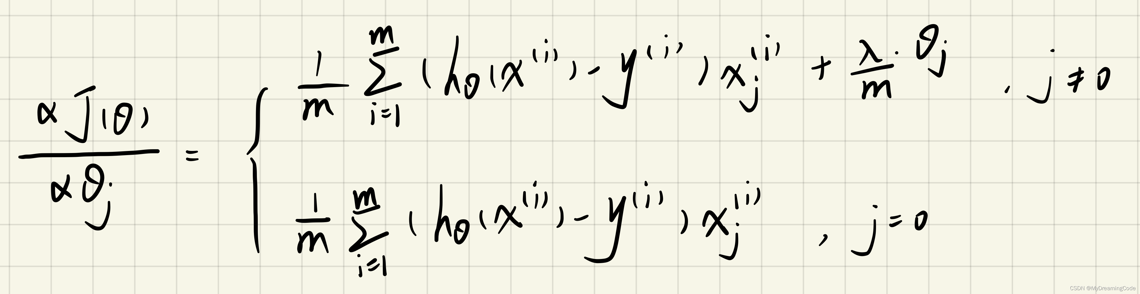
内容：求正则化线性回归的梯度。

gradientReg.py

import numpy as np

def gradientReg(theta, X, y, learningRate):
    m = X.shape[0]
    X = np.matrix(X)
    X = np.insert(X, 0, np.ones(m), axis=1)
    y = np.matrix(y)
    theta = np.matrix(theta)
    grad = (((X * theta.T - y).T * X).T + learningRate * theta.T) / m
    grad[0] = (X * theta.T - y).T * X[:, 0] / m
    return grad

main.py

from scipy.io import loadmat  # 导入matlab格式数据
from gradientReg import *  # 正则化线性回归的梯度

data = loadmat('ex5data.mat')
X, y, Xval, yval, Xtest, ytest = data['X'], data['y'], data['Xval'], data['yval'], data['Xtest'], data['ytest']
theta = [1, 1]
learningRate = 1
gradient = gradientReg(theta, X, y, learningRate)
print(gradient)
# [[-15.30301567]
#  [598.25074417]]

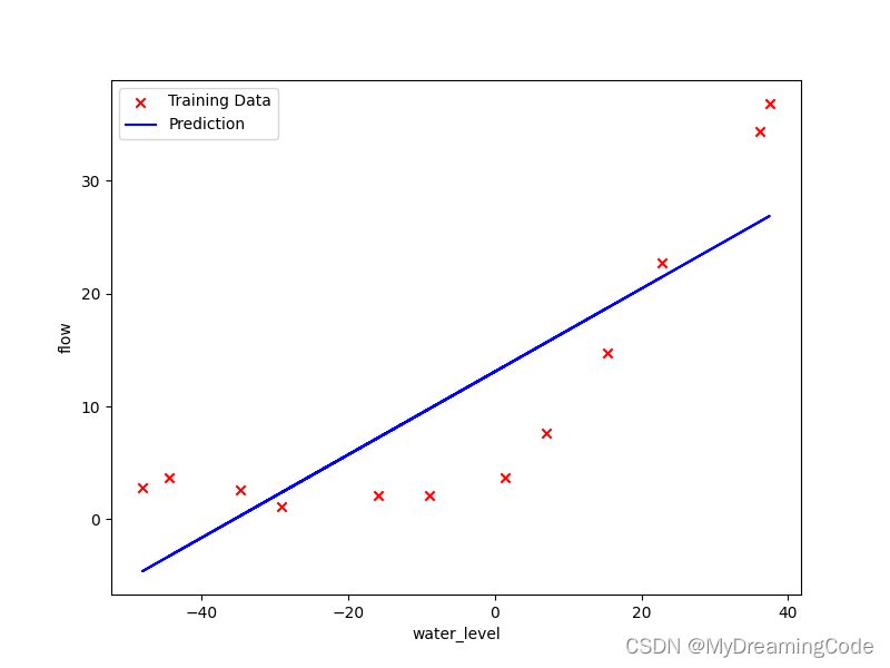
1.4 Fitting linear regression

内容：使用训练好的theta参数，可视化数据和拟合曲线。（因为theta在这里是二维的，正则化对它没有太大的作用，所以在这里可以让 λ=0）

plot.py

import matplotlib.pyplot as plt

def plotTrainingData(X, y):
    fig, ax = plt.subplots(figsize=(8, 6))
    ax.scatter(X, y, marker='x', c='r')
    ax.set_xlabel('water_level')
    ax.set_ylabel('flow')
    plt.show()

def plotHypothesis(theta, X, y):
    fig, ax = plt.subplots(figsize=(8, 6))
    ax.scatter(X, y, c='r', marker='x', label='Training Data')
    ax.plot(X, theta[0] + theta[1] * X, c='b', label='Prediction')
    ax.set_xlabel('water_level')
    ax.set_ylabel('flow')
    ax.legend()
    plt.show()

main.py

from scipy.io import loadmat  # 导入matlab格式数据
import numpy as np
from scipy.optimize import minimize  # 优化
from linearRegCostFunction import *  # 代价函数
from gradientReg import *  # 梯度
from plot import *  # 绘制拟合曲线

data = loadmat('ex5data.mat')
X, y, Xval, yval, Xtest, ytest = data['X'], data['y'], data['Xval'], data['yval'], data['Xtest'], data['ytest']
theta = np.ones(X.shape[1] + 1)
final_theta = minimize(fun=linearRegCostFunction, x0=theta, args=(X, y, 0), method='TNC', jac=gradientReg)['x']
# print(final_theta)  # [13.08790348  0.36777923]
plotHypothesis(final_theta, X, y)

2. Bias-Variance

内容：偏差与方差需要权衡，因为高偏差容易欠拟合，高方差容易过拟合，我们会绘制出学习曲线，来诊断高偏差或是高方差的问题。

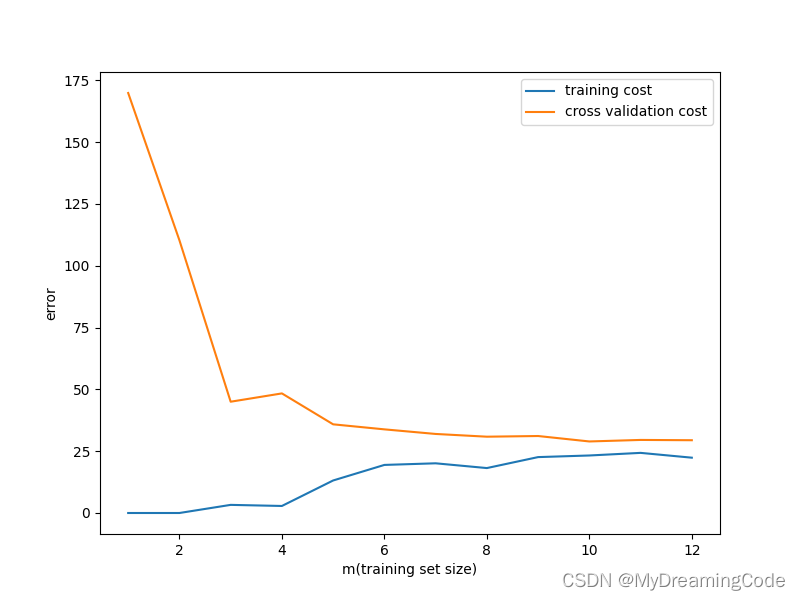
2.1 Learning curves

内容：

（1）函数的自变量为训练集的子集；

（2）训练代价与验证集代价（无需正则化）：

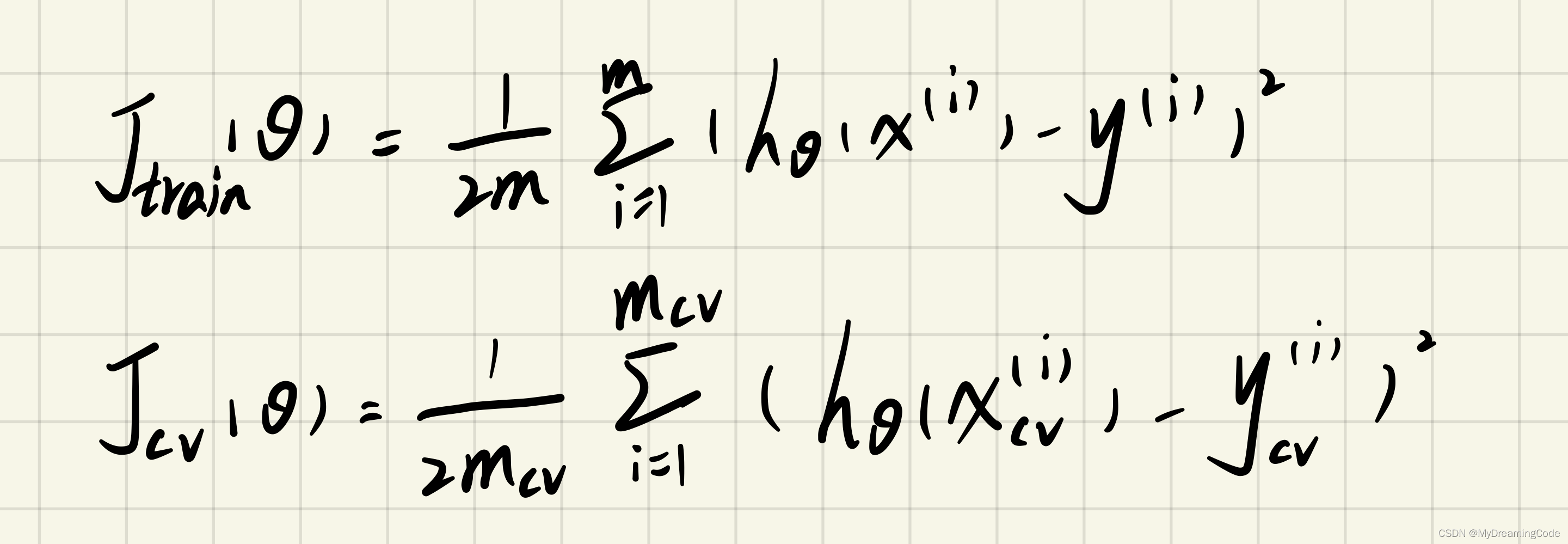
linearRegression.py

import numpy as np
from scipy.optimize import minimize
from linearRegCostFunction import *  # 代价函数
from gradientReg import *  # 梯度

def linearRegression(X, y, learningRate=1):
    theta = np.ones(X.shape[1] + 1)
    res = minimize(fun=linearRegCostFunction, x0=theta, args=(X, y, learningRate), method='TNC', jac=gradientReg)
    return res.x

learningCurve.py

from linearRegression import *  # 线性回归
from linearRegCostFunction import *  # 计算代价函数
from plot import *  # 绘制学习曲线

def learningCurve(X, y, Xval, yval):
    m = X.shape[0]
    train_cost = []
    cv_cost = []
    for i in range(1, m + 1):
        # 随着训练集大小的不断增加，求出对应的最好的theta(能够使代价函数最小)
        res = linearRegression(X[:i, :], y[:i], 0)
        t = linearRegCostFunction(res, X[:i, :], y[:i], 0)
        cv = linearRegCostFunction(res, Xval, yval, 0)
        train_cost.append(t)
        cv_cost.append(cv)
    plotLearningCurve(X, train_cost, cv_cost)

plot.py

import matplotlib.pyplot as plt
import numpy as np

def plotTrainingData(X, y):
    fig, ax = plt.subplots(figsize=(8, 6))
    ax.scatter(X, y, marker='x', c='r')
    ax.set_xlabel('water_level')
    ax.set_ylabel('flow')
    plt.show()

def plotHypothesis(theta, X, y):
    fig, ax = plt.subplots(figsize=(8, 6))
    ax.scatter(X, y, c='r', marker='x', label='Training Data')
    ax.plot(X, theta[0] + theta[1] * X, c='b', label='Prediction')
    ax.set_xlabel('water_level')
    ax.set_ylabel('flow')
    ax.legend()
    plt.show()

def plotLearningCurve(X, train_cost, cv_cost):
    m = X.shape[0]
    fig, ax = plt.subplots(figsize=(8, 6))
    ax.plot(np.arange(1, m + 1), train_cost, label='training cost')
    ax.plot(np.arange(1, m + 1), cv_cost, label='cross validation cost')
    ax.legend()
    ax.set_xlabel('m(training set size)')
    ax.set_ylabel('error')
    plt.show()

main.py

from scipy.io import loadmat  # 导入matlab格式数据
from learningCurve import *  # 学习曲线

data = loadmat('ex5data.mat')
X, y, Xval, yval, Xtest, ytest = data['X'], data['y'], data['Xval'], data['yval'], data['Xtest'], data['ytest']
learningCurve(X, y, Xval, yval)

高偏差（欠拟合）的情况： 

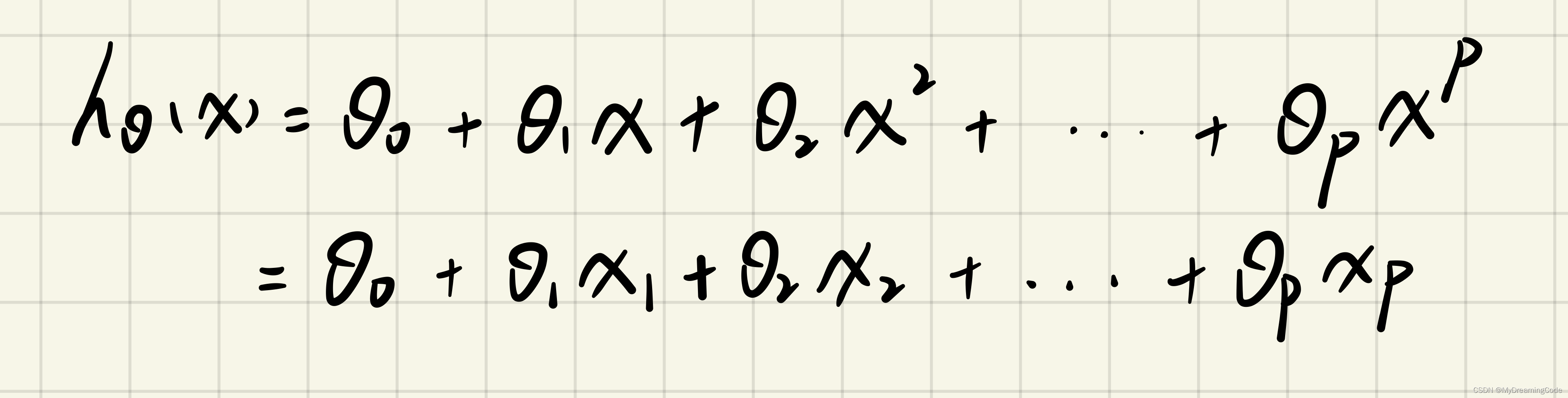
3. Polynomial regression

内容：线性回归模型对于数据的拟合有些差，容易出现欠拟合现象，我们需要再添加一些特征。

polyFeatures.py

import pandas as pd  # 一种用于数据分析的扩展程序库
import numpy as np

def polyFeatures(X, power):
    # 注意F(i)的每一个对应值可以是一个一维数组，所以用ravel进行展开
    data = {"F{}".format(i): np.power(X.ravel(), i) for i in range(1, power + 1)}
    df = pd.DataFrame(data)
    print(df)

main.py

from scipy.io import loadmat  # 导入matlab格式数据
from polyFeatures import *  # 增加特征

data = loadmat('ex5data.mat')
X, y, Xval, yval, Xtest, ytest = data['X'], data['y'], data['Xval'], data['yval'], data['Xtest'], data['ytest']
polyFeatures(X, 3)

           F1           F2             F3
0  -15.936758   253.980260   -4047.621971
1  -29.152979   849.896197  -24777.006175
2   36.189549  1309.683430   47396.852168
3   37.492187  1405.664111   52701.422173
4  -48.058829  2309.651088 -110999.127750
5   -8.941458    79.949670    -714.866612
6   15.307793   234.328523    3587.052500
7  -34.706266  1204.524887  -41804.560890
8    1.389154     1.929750       2.680720
9  -44.383760  1969.918139  -87432.373590
10   7.013502    49.189211     344.988637
11  22.762749   518.142738   11794.353058

3.1 Learning Polynomial Regression

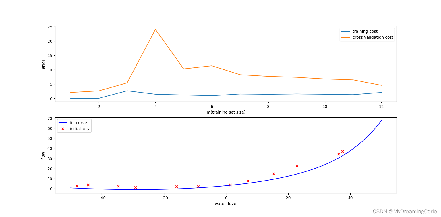
内容：

1. 将特征扩展到8阶（继续视为线性回归的处理方式）；

2. 对特征进行规范化处理；

3. 计算训练集代价与验证集代价并画出学习曲线。

normalizeFeatures.py

def normalizeFeatures(feature):
    # DataFrame.apply(func,axis=0,...)
    # 1.func:函数或lambda表达式,应用于每行或每列
    # 2.lambda表达式:函数式编程，使得apply处理数据时，参数可以传递给函数
    # 3.axis:0(默认值)、index-处理每一列;1、columns-处理每一行
    # 4.规范化处理:减去平均值，再除以标准差(np.std(..))
    return feature.apply(lambda x: (x - x.mean()) / x.std())

polyFeatures.py

import pandas as pd  # 一种用于数据分析的扩展程序库
import numpy as np
from normalizeFeatures import *  # 特征规范化

def polyFeatures(X, power):
    # 注意F(i)的每一个对应值可以是一个一维数组，所以用ravel进行展开
    data = {"F{}".format(i): np.power(X.ravel(), i) for i in range(1, power + 1)}
    df = pd.DataFrame(data)
    new_features = normalizeFeatures(df).values
    return new_features

main.py

from scipy.io import loadmat  # 导入matlab格式数据
from polyFeatures import *  # 增加特征

data = loadmat('ex5data.mat')
X, y, Xval, yval, Xtest, ytest = data['X'], data['y'], data['Xval'], data['yval'], data['Xtest'], data['ytest']
X_poly = polyFeatures(X, 8)  # 训练集扩充特征
Xval_poly = polyFeatures(Xval, 8)  # 验证集扩充特征
print(X_poly[:3, :])

[[-3.62140776e-01 -7.55086688e-01  1.82225876e-01 -7.06189908e-01
   3.06617917e-01 -5.90877673e-01  3.44515797e-01 -5.08481165e-01]
 [-8.03204845e-01  1.25825266e-03 -2.47936991e-01 -3.27023420e-01
   9.33963187e-02 -4.35817606e-01  2.55416116e-01 -4.48912493e-01]
 [ 1.37746700e+00  5.84826715e-01  1.24976856e+00  2.45311974e-01
   9.78359696e-01 -1.21556976e-02  7.56568484e-01 -1.70352114e-01]]

plot.py

import matplotlib.pyplot as plt
import numpy as np
from linearRegression import *  # 得到最优theta
from linearRegCostFunction import *  # 计算代价函数
from polyFeatures import *  # 增加特征

def plotTrainingData(X, y):
    fig, ax = plt.subplots(figsize=(8, 6))
    ax.scatter(X, y, marker='x', c='r')
    ax.set_xlabel('water_level')
    ax.set_ylabel('flow')
    plt.show()

def plotHypothesis(theta, X, y):
    fig, ax = plt.subplots(figsize=(8, 6))
    ax.scatter(X, y, c='r', marker='x', label='Training Data')
    ax.plot(X, theta[0] + theta[1] * X, c='b', label='Prediction')
    ax.set_xlabel('water_level')
    ax.set_ylabel('flow')
    ax.legend()
    plt.show()

def plotLearningCurve(X, train_cost, cv_cost):
    m = X.shape[0]
    fig, ax = plt.subplots(figsize=(8, 6))
    ax.plot(np.arange(1, m + 1), train_cost, label='training cost')
    ax.plot(np.arange(1, m + 1), cv_cost, label='cross validation cost')
    ax.legend()
    ax.set_xlabel('m(training set size)')
    ax.set_ylabel('error')
    plt.show()

def plotPolyLearningCurve(X, y, X_poly, Xval_poly, yval, learningRate):
    train_cost = []
    cv_cost = []
    m = X.shape[0]
    for i in range(1, m + 1):
        res = linearRegression(X_poly[:i, :], y[:i], 0)  # 此时lambda=0可能会出现高方差，即过拟合现象。
        t = linearRegCostFunction(res, X_poly[:i, :], y[:i], 0)
        cv = linearRegCostFunction(res, Xval_poly[:i, :], yval[:i], 0)
        train_cost.append(t)
        cv_cost.append(cv)
    fig, ax = plt.subplots(2, 1, figsize=(8, 8))  # 子图:2行1列 即2*1=2个子图
    # 1.绘制学习曲线
    ax[0].plot(np.arange(1, m + 1), train_cost, label='training cost')
    ax[0].plot(np.arange(1, m + 1), cv_cost, label='cross validation cost')
    ax[0].set_xlabel('m(training set size)')
    ax[0].set_ylabel('error')
    ax[0].legend()
    # 2.绘制拟合曲线
    # a.np.linspace(a,b,c)生成[a,b)之间元素个数为c的序列
    x = np.linspace(-50, 50, 100)
    new_X_poly = np.insert(polyFeatures(x, 8), 0, np.ones(len(x)), axis=1)
    h_theta = new_X_poly * np.matrix(linearRegression(X_poly, y, 0)).T
    ax[1].plot(x, h_theta, c='b', label='fit_curve')
    ax[1].scatter(X, y, c='r', marker='x', label='initial_x_y')
    ax[1].set_xlabel('water_level')
    ax[1].set_ylabel('flow')
    ax[1].legend()
    plt.show()

main.py

from scipy.io import loadmat  # 导入matlab格式数据
from plot import *  # 绘制多项式的拟合曲线以及学习曲线

data = loadmat('ex5data.mat')
X, y, Xval, yval, Xtest, ytest = data['X'], data['y'], data['Xval'], data['yval'], data['Xtest'], data['ytest']
X_poly = polyFeatures(X, 8)  # 训练集扩充特征
Xval_poly = polyFeatures(Xval, 8)  # 验证集扩充特征
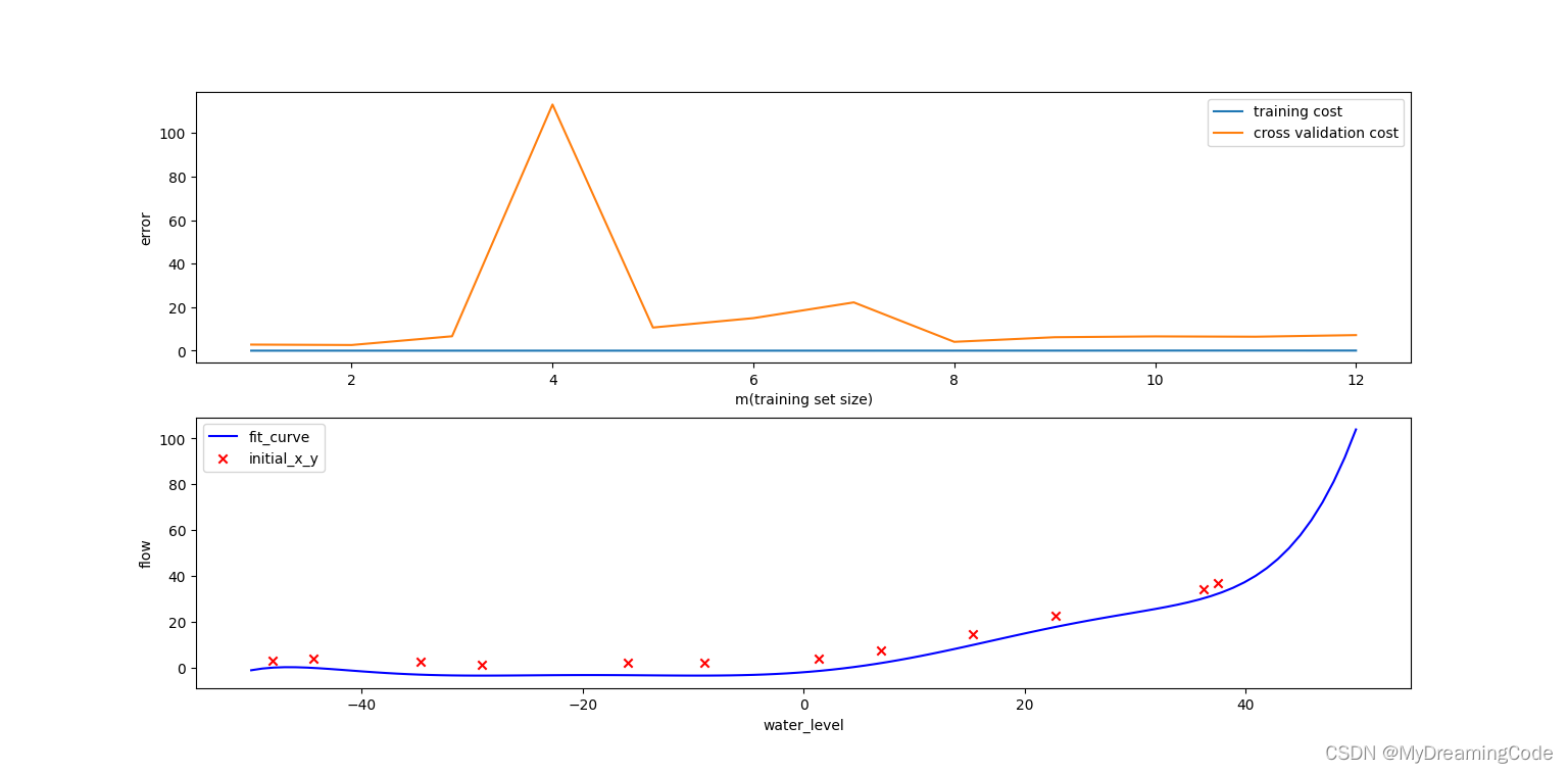
plotPolyLearningCurve(X, y, X_poly, Xval_poly, yval, learningRate=0)

高方差（过拟合）的情况：

3.2 Adjusting the regularization parameter

内容：调整正则化的系数lambda。

A. lambda=1（即learningRate=1）的情况：

plot.py（部分代码）：

def plotPolyLearningCurve(X, y, X_poly, Xval_poly, yval, learningRate):
    train_cost = []
    cv_cost = []
    m = X.shape[0]
    for i in range(1, m + 1):
        res = linearRegression(X_poly[:i, :], y[:i], learningRate)  # 此时lambda=0可能会出现高方差，即过拟合现象。
        t = linearRegCostFunction(res, X_poly[:i, :], y[:i], 0)
        cv = linearRegCostFunction(res, Xval_poly[:i, :], yval[:i], 0)
        train_cost.append(t)
        cv_cost.append(cv)
    fig, ax = plt.subplots(2, 1, figsize=(8, 8))  # 子图:2行1列 即2*1=2个子图
    # 1.绘制学习曲线
    ax[0].plot(np.arange(1, m + 1), train_cost, label='training cost')
    ax[0].plot(np.arange(1, m + 1), cv_cost, label='cross validation cost')
    ax[0].set_xlabel('m(training set size)')
    ax[0].set_ylabel('error')
    ax[0].legend()
    # 2.绘制拟合曲线
    # a.np.linspace(a,b,c)生成[a,b)之间元素个数为c的序列
    x = np.linspace(-50, 50, 100)
    new_X_poly = np.insert(polyFeatures(x, 8), 0, np.ones(len(x)), axis=1)
    h_theta = new_X_poly * np.matrix(linearRegression(X_poly, y, learningRate)).T
    ax[1].plot(x, h_theta, c='b', label='fit_curve')
    ax[1].scatter(X, y, c='r', marker='x', label='initial_x_y')
    ax[1].set_xlabel('water_level')
    ax[1].set_ylabel('flow')
    ax[1].legend()
    plt.show()

main.py（修改一句）

plotPolyLearningCurve(X, y, X_poly, Xval_poly, yval, learningRate=1) 

在学习曲线中可以看到，训练集的代价不再是0，即我们减轻了过拟合。 

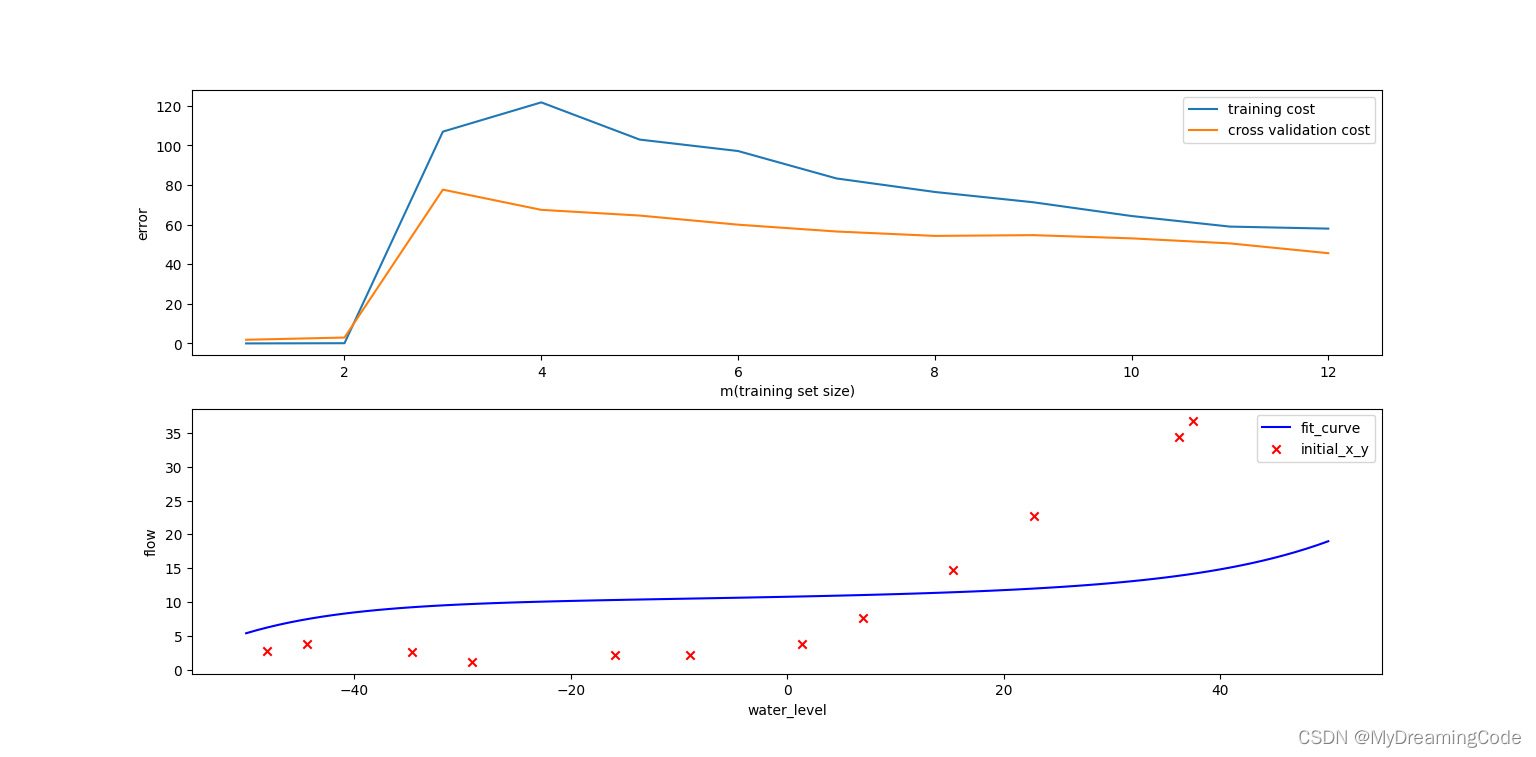
B. lambda=100（即learningRate=100）的情况：

main.py（修改一句）

plotPolyLearningCurve(X, y, X_poly, Xval_poly, yval, learningRate=100) 

lambda惩罚项太大，出现了欠拟合的情况：

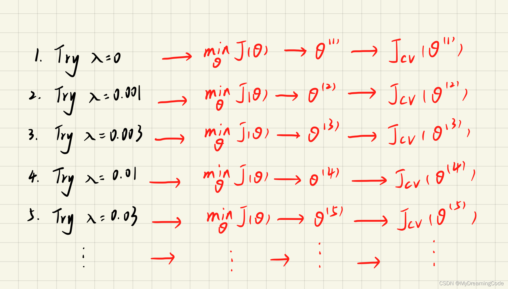
3.3 Selecting λ using a cross validation set 

内容：使用验证集来评价 λ 的好坏，选择好的 λ 后，在测试集上进行测试。lambda可以尝试0,0.001,0.003,0.01,0.03,0.1,0.3,1,3,10这些值。

chooseLambda.py

from plot import *  # 绘制lambda与代价函数(训练集、验证集)的图像

def chooseLambda(X_poly, y, Xval_poly, yval):
    l_candidate = [0, 0.001, 0.003, 0.01, 0.03, 0.1, 0.3, 1, 3, 10]  # lambda候选值
    train_cost = []
    cv_cost = []
    for l in l_candidate:
        res = linearRegression(X_poly, y, l)
        train_cost.append(linearRegCostFunction(res, X_poly, y, 0))
        cv_cost.append(linearRegCostFunction(res, Xval_poly, yval, 0))
    plotChooseLambda(l_candidate, train_cost, cv_cost)

plot.py（增加一个函数）

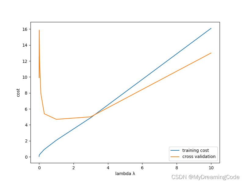
def plotChooseLambda(l_candidate, train_cost, cv_cost):
    fig, ax = plt.subplots(figsize=(8, 6))
    ax.plot(l_candidate, train_cost, label='training cost')
    ax.plot(l_candidate, cv_cost, label='cross validation')
    ax.set_xlabel('lambda λ')
    ax.set_ylabel('cost')
    ax.legend()
    plt.show()

main.py

from scipy.io import loadmat  # 导入matlab格式数据
from chooseLambda import *  # 选择最合适的lambda

data = loadmat('ex5data.mat')
X, y, Xval, yval, Xtest, ytest = data['X'], data['y'], data['Xval'], data['yval'], data['Xtest'], data['ytest']
X_poly = polyFeatures(X, 8)  # 训练集扩充特征
Xval_poly = polyFeatures(Xval, 8)  # 验证集扩充特征
chooseLambda(X_poly, y, Xval_poly, yval)

cross validation的最小值在4附近，对应的lambda值约为1。 

3.4 Computing test set error

内容：在测试集（之前从未被使用过的数据）上做评估。

testSet.py

from linearRegression import *  # 计算出最优theta
from linearRegCostFunction import *  # 计算代价函数

def testSet(X_poly, y, Xtest_poly, ytest):
    l_candidate = [0, 0.001, 0.003, 0.01, 0.03, 0.1, 0.3, 1, 3, 10]  # lambda候选值
    for l in l_candidate:
        theta = linearRegression(X_poly, y, l)
        print("test cost(l={})={}".format(l, linearRegCostFunction(theta, Xtest_poly, ytest, l)))

main.py

from scipy.io import loadmat  # 导入matlab格式数据
from polyFeatures import *  # 扩展特征
from testSet import *  # 在测试集上应用

data = loadmat('ex5data.mat')
X, y, Xval, yval, Xtest, ytest = data['X'], data['y'], data['Xval'], data['yval'], data['Xtest'], data['ytest']
X_poly = polyFeatures(X, 8)
Xtest_poly = polyFeatures(Xtest, 8)
testSet(X_poly, y, Xtest_poly, ytest)

test cost(l=0)=10.088273811962134
test cost(l=0.001)=10.936688556161654
test cost(l=0.003)=11.22874602267731
test cost(l=0.01)=10.992356113176701
test cost(l=0.03)=10.026774833897209
test cost(l=0.1)=8.624697841922986
test cost(l=0.3)=7.336693296833649
test cost(l=1)=7.477384083967169
test cost(l=3)=11.645564884360581
test cost(l=10)=27.71507101822064

此时，λ=0.3测得的代价函数最小，故λ=0.3为最优选择。