


import pandas as pd
import numpy as np
import matplotlib.pylab as plt
import warnings
warnings.filterwarnings('ignore')

#设置中文字体
plt.rcParams['font.sans-serif']=['SimHei']
plt.rcParams['axes.unicode_minus']=False

#读取excel文件
def load_parking_data(filepath):
    try:
        df=pd.read_excel(file_path)
        print('数据加载成功!')
        print(f'数据形状:{df.shape}')
        print('\n数据前5行:')
        print(df.head())
        print('数据基本信息:')
        print(df.info())
        return df
    except Exception as e:
        print(f'读取文件出错:{e}')
        return None
#加载数据
file_path='停车场信息表.xlsx'
parking_df=load_parking_data(file_path)
数据加载成功!
数据形状:(9281, 6)

数据前5行:
        cn               timein              timeout  price  state  rps
0  赣CFF120  2018-01-01 00:03:13  2018-01-01 00:23:52      3      1   99
1  云N84SU5  2018-01-01 00:09:37  2018-01-01 00:44:54      3      1   99
2  冀RLDH16  2018-01-01 00:38:08  2018-01-01 00:45:29      3      1  100
3  豫K869CW  2018-01-01 00:52:53  2018-01-01 00:59:04      3      1  100
4  新QWWA64  2018-01-01 01:20:37  2018-01-01 01:24:10      3      1  100
数据基本信息:
<class 'pandas.core.frame.DataFrame'>
RangeIndex: 9281 entries, 0 to 9280
Data columns (total 6 columns):
 #   Column   Non-Null Count  Dtype
---  ------   --------------  -----
 0   cn       9281 non-null   object
 1   timein   9281 non-null   object
 2   timeout  9281 non-null   object
 3   price    9281 non-null   int64
 4   state    9281 non-null   int64
 5   rps      9281 non-null   int64
dtypes: int64(3), object(3)
memory usage: 435.2+ KB
None
if parking_df is not None:
    parking_df['timein']=pd.to_datetime(parking_df['timein'],errors='coerce')
    parking_df['timeout']=pd.to_datetime(parking_df['timeout'],errors='coerce')
parking_df.describe()
| 时间在 | 超时 | 价格 | 州 | RPS的 | |
|---|---|---|---|---|---|
| 计数 | 9281 | 9279 | 9281.000000 | 9281.000000 | 9281.000000 |
| 意味 着 | 2018-02-15 00:34:30.038896640 | 2018-02-15 04:05:29.693178112 | 11.914988 | 0.999785 | 83.240384 |
| 分钟 | 2018-01-01 00:03:13 | 2018-01-01 00:23:52 | 0.000000 | 0.000000 | 34.000000 |
| 25% | 2018-01-23 15:16:29 | 2018-01-24 02:06:26 | 3.000000 | 1.000000 | 75.000000 |
| 50% | 2018-02-14 10:50:18 | 2018-02-14 13:28:54 | 6.000000 | 1.000000 | 86.000000 |
| 75% | 2018-03-09 06:55:44 | 2018-03-09 08:14:01.500000 | 15.000000 | 1.000000 | 94.000000 |
| 麦克斯 | 2018-03-31 23:35:29 | 2018-03-31 23:51:10 | 105.000000 | 1.000000 | 100.000000 |
| 性病 | 南 | 南 | 13.500056 | 0.014679 | 13.205254 |
1.停车时长分析
def analyze_parking_duration(df):
    # 只分析已驶出的车辆(state=1)
    completed_df=df[df['state']==1].copy()
    # 计算停车时长(分钟)
    completed_df['duration_minustes']=(completed_df['timeout']-completed_df['timein']).dt.total_seconds()/60
    # 转换为小时
    completed_df['duration_hours']=completed_df['duration_minustes']/60
    # 分析统计量
    duration_stats=completed_df['duration_hours'].describe()
    # 可视化
    fig,axes=plt.subplots(2,2,figsize=(8,6))
    fig.suptitle('停车时长分析',fontsize=16,fontweight='bold')
    # 停车时长分布的直方图
    axes[0,0].hist(completed_df['duration_hours'],bins=50,edgecolor='black',alpha=0.7,color='skyblue')
    axes[0,0].set_xlabel('停车时长(小时)')
    axes[0,0].set_ylabel('频次')
    axes[0,0].set_title('停车时长分布')
    axes[0,0].grid(True,alpha=0.3)

    # 时长的箱线图
    axes[0,1].boxplot(completed_df['duration_hours'])
    axes[0,1].set_ylabel('停车时长分布')
    axes[0,1].set_title('停车时长箱线图')
    axes[0,1].grid(True,alpha=0.3)

    #市场分布(0-24小时)
    short_duration=completed_df[completed_df['duration_hours']<=24]['duration_hours']
    axes[1,0].hist(short_duration,bins=50,edgecolor='black',alpha=0.7,color='lightgreen')
    axes[1,0].set_xlabel('停车时长(小时,0-24小时)')
    axes[1,0].set_ylabel('频次')
    axes[1,0].set_title('24小时内停车时长分布')
    axes[1,0].grid(True,alpha=0.3)

    #时长百分比分布
    duration_categories=pd.cut(completed_df['duration_hours'],
                                bins=[0,1,3,6,12,24,48,np.inf],  #分箱
                                labels=['<1h','1-3h','3-6h','6-12h','12-24h','24-48h','>48h'])
    category_counts=duration_categories.value_counts().sort_index()
    axes[1,1].bar(range(len(category_counts)),category_counts.values,alpha=0.7)
    axes[1,1].set_xlabel('停车时长(区间)')
    axes[1,1].set_ylabel('车辆数量')
    axes[1,1].set_title('停车时长区间分布')
    axes[1,1].set_xticks(range(len(category_counts)))
    axes[1,1].set_xticklabels(category_counts.index,rotation=45)
    axes[1,1].grid(True,alpha=0.3)
    # 添加数值标签
    for i,v in enumerate(category_counts.values):
        axes[1,1].text(i,v+5,str(v),ha='center',va='bottom')
    plt.tight_layout()
    plt.show()
    print('停车时长统计')
    print(duration_stats)
    print('停车时长区间分布')
    print(category_counts)
    return duration_stats,completed_df
print('='*50)
print('停车时长分析')
print('='*50)
duration_stats,comletted_df=analyze_parking_duration(parking_df)
==================================================
停车时长分析
==================================================
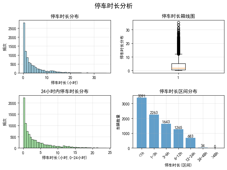
停车时长统计
count    9279.000000
mean        3.748868
std         4.649420
min         0.000278
25%         0.514444
50%         1.874722
75%         5.153750
max        35.227500
Name: duration_hours, dtype: float64
停车时长区间分布
duration_hours
<1h       3391
1-3h      2263
3-6h      1643
6-12h     1265
12-24h     683
24-48h      34
>48h         0
Name: count, dtype: int64
2-3. 停车高峰时间统计、周每天停车统计
def analyze_peak_hours(df):
    # 提取进入时间的小时和星期几
    df['hour_in'] = df['timein'].dt.hour
    df['day_of_week'] = df['timein'].dt.dayofweek  # 周一=0,周日=6
    df['day_name'] = df['timein'].dt.day_name()

    # 按小时统计进入车辆
    hourly_count = df.groupby('hour_in').size()
    # 按星期统计进入车辆数
    daily_count = df.groupby('day_of_week').size()

    # 可视化
    fig, axes = plt.subplots(2, 2, figsize=(8, 6))
    fig.suptitle('停车高峰时间分析', fontsize=16, fontweight='bold')

    # 小时分布
    axes[0, 0].bar(hourly_count.index, hourly_count.values, alpha=0.7, color='skyblue')
    axes[0, 0].set_xlabel('小时')
    axes[0, 0].set_ylabel('进入车辆数')
    axes[0, 0].set_title('各小时进入车辆分布')
    axes[0, 0].set_xticks(range(0, 24))
    axes[0, 0].grid(True, alpha=0.3)

    # 星期分布
    day_names = ['周一', '周二', '周三', '周四', '周五', '周六', '周日']
    axes[0, 1].bar(daily_count.index, daily_count.values, alpha=0.7, color='lightcoral')
    axes[0, 1].set_xlabel('星期')
    axes[0, 1].set_ylabel('进入车辆数')
    axes[0, 1].set_title('各星期进入车辆分布')
    axes[0, 1].set_xticks(range(0, 7))
    axes[0, 1].set_xticklabels(day_names)
    axes[0, 1].grid(True, alpha=0.3)

    # 按时间段统计
    time_bins = [0, 6, 9, 12, 17, 20, 24]
    time_labels = ['深夜(0-6)', '早高峰(6-9)', '上午(9-12)', '下午(12-15)',
                   '晚高峰(17-20)', '夜晚(20-24)']
    df['time_period'] = pd.cut(df['hour_in'], bins=time_bins,
                              labels=time_labels, right=False)
    period_count = df.groupby('time_period').size()

    # 饼图颜色列表修正
    colors = ['lightblue', 'lightcoral', 'lightgreen', 'lightyellow',
             'lightpink', 'lightgray']

    axes[1, 0].pie(period_count.values, labels=period_count.index,
                  autopct='%1.1f%%', colors=colors)
    axes[1, 0].set_title('各时间段进入车辆比例')

    plt.tight_layout()
    plt.show()

    # 找出高峰时段
    peak_hour = hourly_count.idxmax()
    peak_day = daily_count.idxmax()

    print('高峰时间分析结果:')
    print(f'最繁忙小时: {peak_hour}时, 车辆数: {hourly_count.max()}')
    print(f'最繁忙星期: {day_names[peak_day]}, 车辆数: {daily_count.max()}')
    print('各时间段车辆分析')
    for period, count in period_count.items():
        print(f'{period}: {count}辆({count/len(df)*100:.1f}%)')

    return hourly_count, daily_count, period_count
print('='*50)
print('停车高峰时间分析')
print('='*50)
hourly_count,daily_count,period_count=analyze_peak_hours(parking_df)
==================================================
停车高峰时间分析
==================================================
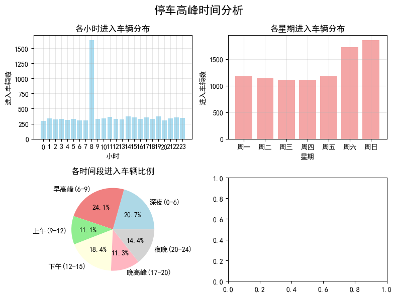
高峰时间分析结果:
最繁忙小时: 8时, 车辆数: 1631
最繁忙星期: 周日, 车辆数: 1853
各时间段车辆分析
深夜(0-6): 1918辆(20.7%)
早高峰(6-9): 2240辆(24.1%)
上午(9-12): 1032辆(11.1%)
下午(12-15): 1704辆(18.4%)
晚高峰(17-20): 1050辆(11.3%)
夜晚(20-24): 1337辆(14.4%)
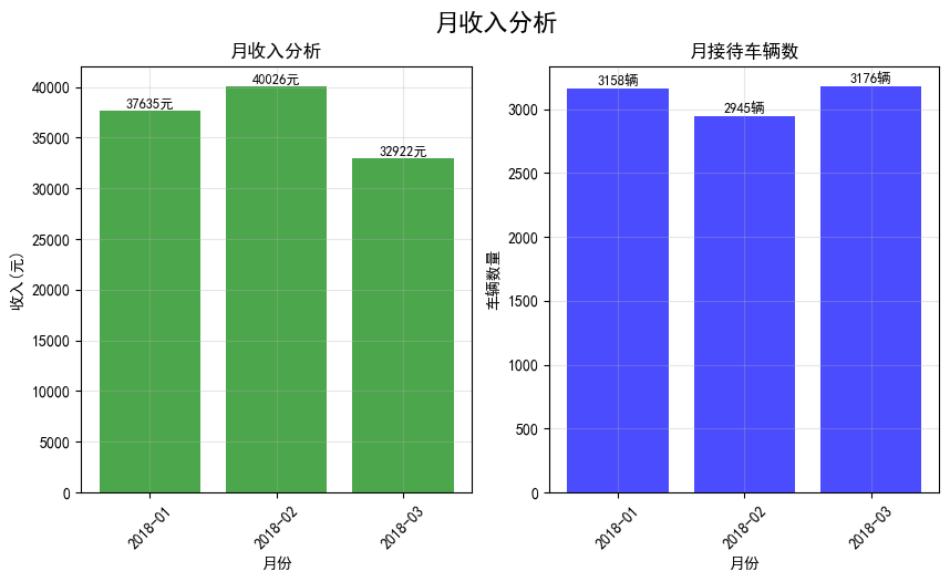
4.月收入分析
# 4.月收入分析
def analyze_monthly_income(df):
    #只分析已经缴费的车辆
    paid_df=df[df['state']==1].copy()

    #提取年月信息
    paid_df['year_month']=paid_df['timein'].dt.to_period('M')

    #按月统计收入
    monthly_income=paid_df.groupby('year_month')['price'].sum()
    #统计车辆
    monthly_count=paid_df.groupby('year_month').size()

    #计算平均每车收入
    avg_income_per_car=monthly_income/monthly_count

    #可视化
    fig,axes=plt.subplots(1,2,figsize=(10,5))
    fig.suptitle('月收入分析',fontsize=16,fontweight='bold')
    #月收入柱状图
    axes[0].bar(range(len(monthly_income)),monthly_income.values,alpha=0.7,color='green')
    axes[0].set_xlabel('月份')
    axes[0].set_ylabel('收入(元)')
    axes[0].set_title('月收入分析')
    axes[0].set_xticks(range(len(monthly_income)))
    axes[0].set_xticklabels([str(ym) for ym in monthly_income.index],rotation=45)
    axes[0].grid(True,alpha=0.3)
    #在柱子上添加数值标签
    for i,v in enumerate(monthly_income.values):
        axes[0].text(i,v+100,f'{v:.0f}元',ha='center',va='bottom',size=9)

    #月接待数量
    axes[1].bar(range(len(monthly_count)),monthly_count.values,alpha=0.7,color='blue')
    axes[1].set_xlabel('月份')
    axes[1].set_ylabel('车辆数量')
    axes[1].set_title('月接待车辆数')
    axes[1].set_xticks(range(len(monthly_count)))
    axes[1].set_xticklabels([str(ym) for ym in monthly_income.index],rotation=45)
    axes[1].grid(True,alpha=0.3)
    for i,v in enumerate(monthly_count.values):
        axes[1].text(i,v+10,f'{v}辆',ha='center',va='bottom',size=9)

    return monthly_income,monthly_count,avg_income_per_car
print('='*50)
print('月收入分析')
print('='*50)
monthly_income,monthly_count,avg_income_per_car=analyze_monthly_income(parking_df)
==================================================
月收入分析
==================================================
5.每日接待车辆统计
def analyze_daily_traffic(df):
    # 提取日期信息
    df['date'] = df['timein'].dt.date

    # 按日期统计车辆数量
    daily_count = df.groupby('date').size()

    # 可视化
    fig, axes = plt.subplots(1, 2, figsize=(12, 5))
    fig.suptitle('每日接待车辆统计', fontsize=16, fontweight='bold')

    # 每日车辆数量折线图
    axes[0].plot(range(len(daily_count)), daily_count.values, marker='o', linestyle='-', color='blue', alpha=0.7)
    axes[0].set_xlabel('日期')
    axes[0].set_ylabel('车辆数量')
    axes[0].set_title('每日接待车辆趋势')
    axes[0].set_xticks(range(0, len(daily_count), 5))  # 每5天显示一个刻度
    axes[0].set_xticklabels([str(date) for i, date in enumerate(daily_count.index) if i % 5 == 0], rotation=45)
    axes[0].grid(True, alpha=0.3)

    # 每日车辆数量分布直方图
    axes[1].hist(daily_count.values, bins=20, edgecolor='black', alpha=0.7, color='orange')
    axes[1].set_xlabel('每日车辆数量')
    axes[1].set_ylabel('天数')
    axes[1].set_title('每日车辆数量分布')
    axes[1].grid(True, alpha=0.3)

    # 添加统计信息
    mean_count = daily_count.mean()
    max_count = daily_count.max()
    min_count = daily_count.min()
    axes[1].axvline(mean_count, color='red', linestyle='--', label=f'平均值: {mean_count:.1f}')
    axes[1].axvline(max_count, color='green', linestyle='--', label=f'最大值: {max_count}')
    axes[1].axvline(min_count, color='blue', linestyle='--', label=f'最小值: {min_count}')
    axes[1].legend()

    plt.tight_layout()
    plt.show()

    # 输出统计信息
    print('每日接待车辆统计:')
    print(f'总天数: {len(daily_count)}天')
    print(f'平均每日车辆: {mean_count:.1f}辆')
    print(f'最大日车辆: {max_count}辆 (日期: {daily_count.idxmax()})')
    print(f'最小日车辆: {min_count}辆 (日期: {daily_count.idxmin()})')
    print(f'总车辆数: {daily_count.sum()}辆')

    return daily_count
print('='*50)
print('每日接待车辆统计')
print('='*50)
daily_count = analyze_daily_traffic(parking_df)
==================================================
每日接待车辆统计
==================================================
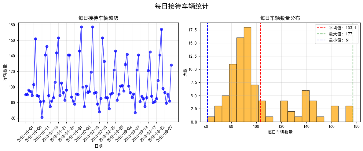
每日接待车辆统计:
总天数: 90天
平均每日车辆: 103.1辆
最大日车辆: 177辆 (日期: 2018-02-04)
最小日车辆: 61辆 (日期: 2018-01-11)
总车辆数: 9281辆
6.车位利用率分析
def daily_utilization_analyze(df, total_spaces=100):
    # 按日期分组
    df['date'] = df['timein'].dt.date
    daily_stats = df.groupby('date').agg({
        'rps': ['mean', 'min', 'max'],  # 平均、最小、最大空余车位数
        'cn': 'count'  # 车位进出次数
    }).round(2)

    daily_stats.columns = ['avg_rps', 'min_rps', 'max_rps', 'car_count']
    daily_stats['avg_utilization'] = (total_spaces - daily_stats['avg_rps']) / total_spaces * 100
    daily_stats['max_utilization'] = (total_spaces - daily_stats['min_rps']) / total_spaces * 100
    daily_stats['min_utilization'] = (total_spaces - daily_stats['max_rps']) / total_spaces * 100

    # 可视化
    fig, axes = plt.subplots(1, 3, figsize=(15, 5))
    fig.suptitle('车位利用率分析', fontsize=16, fontweight='bold')

    # 平均利用率趋势
    axes[0].plot(daily_stats.index.astype(str),daily_stats['avg_utilization'])
    axes[0].set_title('每日平均车位利用率')
    axes[0].set_xlabel('2018-01-01至2018-03-31')
    axes[0].set_ylabel('利用率(%)')
    axes[0].tick_params(axis='x', rotation=10)
    axes[0].grid(True, alpha=0.3)

    # 最大利用率趋势
    axes[1].plot(daily_stats.index.astype(str),daily_stats['max_utilization'])
    axes[1].set_title('每日最大车位利用率')
    axes[1].set_xlabel('2018-01-01至2018-03-31')
    axes[1].set_ylabel('利用率(%)')
    axes[1].tick_params(axis='x', rotation=10)
    axes[1].grid(True, alpha=0.3)

    # 最小利用率趋势
    axes[2].plot(daily_stats.index.astype(str),daily_stats['min_utilization'])
    axes[2].set_title('每日最小车位利用率')
    axes[2].set_xlabel('2018-01-01至2018-03-31')
    axes[2].set_ylabel('利用率(%)')
    axes[2].tick_params(axis='x', rotation=10)
    axes[2].grid(True, alpha=0.3)

    plt.tight_layout()
    plt.show()

    # 输出统计信息
    print('车位利用率统计:')
    print(f'平均利用率: {daily_stats["avg_utilization"].mean():.1f}%')
    print(f'最高利用率: {daily_stats["max_utilization"].max():.1f}%')
    print(f'最低利用率: {daily_stats["min_utilization"].min():.1f}%')

    return daily_stats
daily_stats = daily_utilization_analyze(parking_df, total_spaces=100)
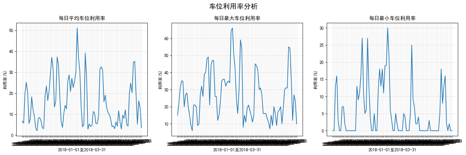
车位利用率统计:
平均利用率: 15.6%
最高利用率: 66.0%
最低利用率: 0.0%


 680
680

 被折叠的 条评论
为什么被折叠?
被折叠的 条评论
为什么被折叠?
 到【灌水乐园】发言


