Task02：回归-优快云博客

本文详细介绍了线性回归模型在房价预测和股市预测中的应用，涉及模型假设（一元/多元线性）、损失函数的选择与梯度下降优化，以及如何通过训练集和测试集验证模型性能。讨论了过拟合问题、模型复杂度提升和正则化的应对策略。

摘要生成于 C知道，由 DeepSeek-R1 满血版支持，前往体验 >

一、定义

Regression就是找到一个函数function，通过输入特征x，得到一个返回值。

二、应用

房价预测
1. 输入：根据房屋面积，地理位置等
2. 输出：预测房屋的价格
股市的预测：
1. 输入：过去10年股票的变动，新闻咨询，公司并购咨询等
2. 输出：预测股市的明天的平均值

三、步骤

1、模型假设（线性模型）

一元线性模型

一元线性模型针对于单个输入特征的情况。以一个特征Xcp为例，此线性模型假设为： $\mathrm{y}=\mathrm{b}+ \mathrm{w} \mathrm{x}$

多元线性模型

在实际生活中，为得到所预测的返回值，往往输入的特征值Xcp不止一个。例如预测房价时，为得到此时房价，我们要考虑到房屋面积，地理位置等因素，特征值往往会很多。
所以㧴们假设线性模型 Linear model: $\mathrm{y}=\mathrm{b}+\sum \mathrm{w}_{\mathrm{i}} \mathrm{x}_{\mathrm{i}}$

$\mathrm{x}_{\mathrm{i}}$ : 就是各种特征(feture)
$\mathrm{w}_{\mathrm{i}}$ : 各个特征的权重
b: 偏移量

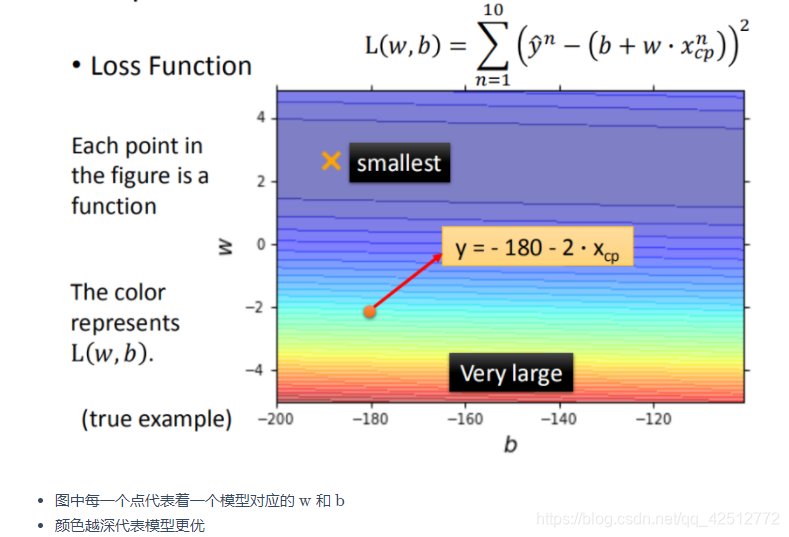
2、模型评估（损失函数）

求取理论值与预测值之间的差值，来判断所找寻的模型的好坏。即引入损失函数（Loss Function），用以衡量模型的好坏。定义损失函数为：
$\mathrm{L}(\mathrm{w}, \mathrm{b})=\sum_{\mathrm{n}=1}^{10}\left(\hat{\mathrm{y}}^{\mathrm{n}}-\left(\mathrm{b}+\mathrm{w} \cdot \mathrm{x}_{\mathrm{cp}}\right)\right)^{2}$
在这里插入图片描述

3、模型优化（梯度下降）

针对损失函数，
$\mathrm{L}(\mathrm{w}, \mathrm{b})=\sum_{\mathrm{n}=1}^{10}\left(\hat{\mathrm{y}}^{\mathrm{n}}-\left(\mathrm{b}+\mathrm{w} \cdot \mathrm{x}_{\mathrm{cp}}\right)\right)^{2}$
需要找到一个零结果最小的 $f^*$ .在实际的场景之中，我们遇到的参数肯定不止w，b。我们要寻找到到一个好的模型，使损失函数达到最小，则：
$\begin{aligned} f^{*}=\arg \min _{f} L(f) & \\ w^{*}, b^{*}=\arg \min _{w, b} L(w, b) & =\arg \min _{w, b} \sum_{n=1}^{10}\left(\hat{y}^{n}-\left(b+w \cdot x_{c p}^{n}\right)\right)^{2} \end{aligned}$

先从最简单的只有一个参数w入手，定义 $w^{*} = \arg \min _{w, b} L(w)$ ，
在这里插入图片描述
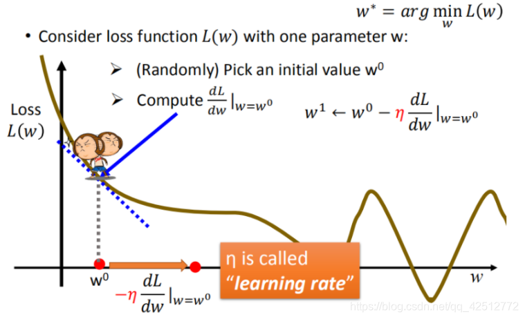
首先在这里引入一个概念学习率：移动的步长，如上图中 $\eta$

步骤1：随机选取一个 $w^0$
步骤2：计算微分，也就是当前的斜率，根据斜率来判定移动的方向
大于0向右移动（增加w）
小于0向左移动（减少w）
步骤3：根据学习率移动
重复步骤2和步骤3，直到找到最低点
在这里插入图片描述

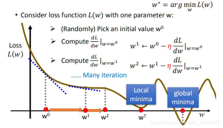
步骤1中，我们随机选取一个 $w^0$ ，如上图所示，我们有可能会找到当前的最小值，并不是全局的最小值。

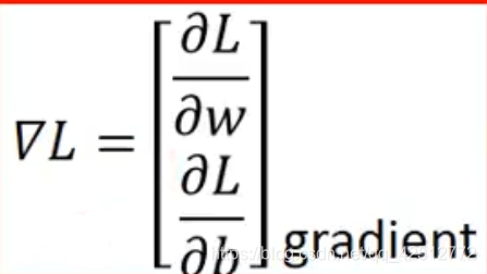
而对于两个变量时，一般的步骤如下图所示。

整理成一个更简洁的公式：
在这里插入图片描述
在梯度下降推演最优化的过程中，如果把w，b在图形中展示

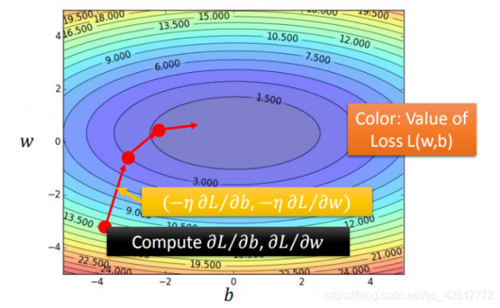
每一条线围成的圈就是等高线，代表损失函数的值，颜色约深的区域代表的损失函数越小。红色的箭头代表等高线的法线方向。

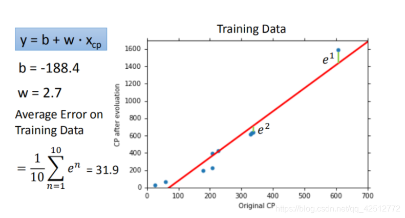
四、如何验证训练模型的好坏

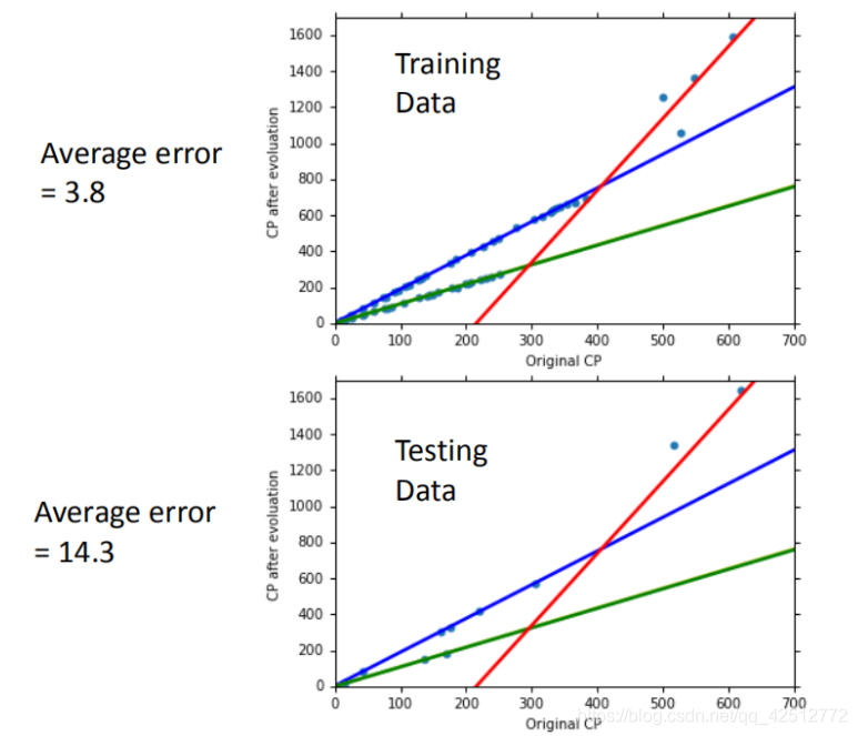
使用训练集和测试集的平均误差来验证模型的好坏我们使用将10组原始数据，训练集求得平均误差为31.9，如图所示：

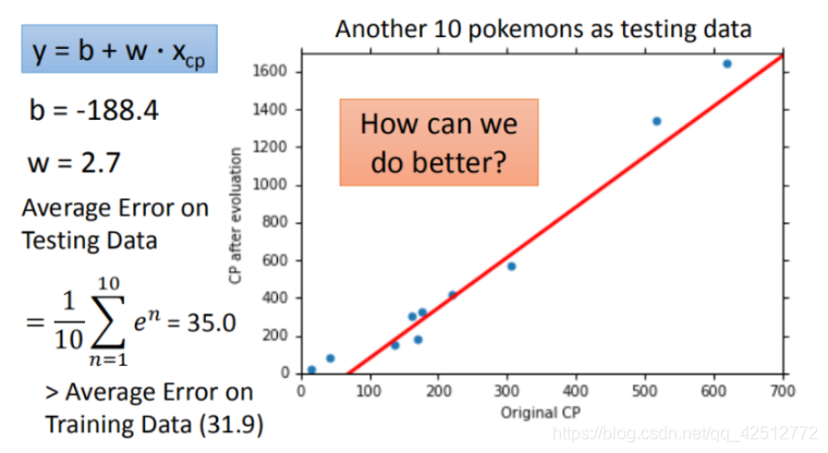
然后再使用10组Pokemons测试模型，测试集求得平均误差为35.0 如图所示：
在这里插入图片描述

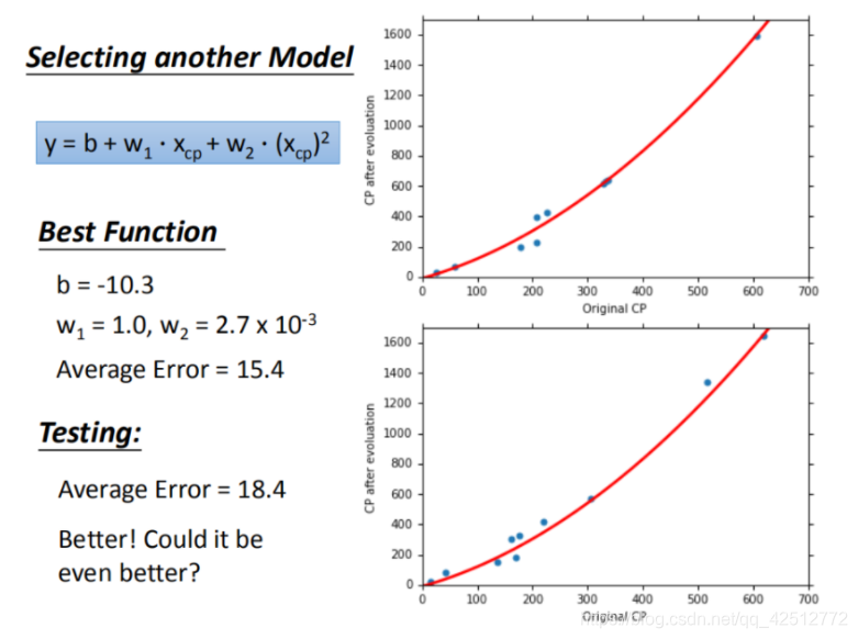
更强大复杂的模型：1元N次线性模型

在模型上，我们还可以进一部优化，选择更复杂的模型，使用1元2次方程举例，如下图，发现训练集求得平均误差为15.4，测试集的平均误差为18.4。
在这里插入图片描述

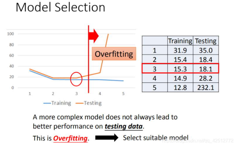
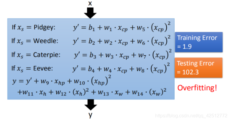
过拟合问题出现

在模型上，使用更高次方的模型进一步优化，但我们会发现在训练集上表现优秀的模型，到了测试集上效果反而变差了。这是因为模拟在训练集上出现了过拟合的问题。

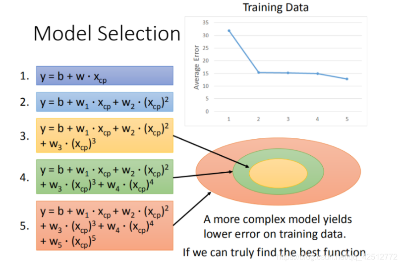
将上述选择的模型所产生的错误率结果进行图形化展示，如下图所示，发现3次方以上的模型，出现了过拟合的现象。
在这里插入图片描述

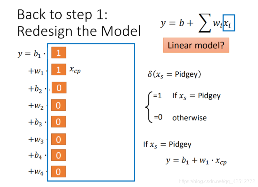
五、步骤优化

1、2个input的四个线性模型合并到一个线性模型中

在这里插入图片描述

2、使用更多的输入

将最开始分析得到的很多特征，都加入到模型当中
在这里插入图片描述

3、加入正则化

更多特征，但是权重 w 可能会使某些特征权值过高，仍旧导致过拟合现象，所以加入正则化。

在这里插入图片描述

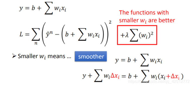
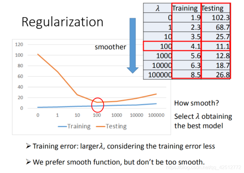
w 越小，表示 functionfunction 较平滑的， functionfunction输出值与输入值相差不大。在很多应用场景中，并不是 w 越小模型越平滑越好，但是经验值告诉我们 w 越小大部分情况下都是好的。b 的值接近于0 ，对曲线平滑是没有影响。

六、代码实现

import numpy as np
import matplotlib.pyplot as plt


x_data = [338., 333., 328., 207., 226., 25., 179., 60., 208., 606.]
y_data = [640., 633., 619., 393., 428., 27., 193., 66., 226., 1591.]
x = np.arange(-200,-100,1)
y = np.arange(-5,5,0.1)
#损失函数
Z = np.zeros((len(x), len(y)))
for i in range(len(x)):
    for j in range(len(y)):
        b = x[i]
        w = y[j]
        Z[j][i] = 0
        for n in range(len(x_data)):
            Z[j][i] = Z[j][i] + (y_data[n] - b - w*x_data[n])**2
        Z[j][i] = Z[j][i] / len(x_data)


def train(lr, iteration):
    # 线性回归原始版
    b = -120
    w = -4

    b_history = [b]
    w_history = [w]

    for i in range(iteration):
        b_grad = 0.0
        w_grad = 0.0
        for n in range(len(x_data)):
            b_grad = b_grad - 2.0 * (y_data[n] - b - w * x_data[n]) * 1.0
            w_grad = w_grad - 2.0 * (y_data[n] - b - w * x_data[n]) * x_data[n]

        # 更新参数
        b -= lr * b_grad
        w -= lr * w_grad

        b_history.append(b)
        w_history.append(w)

    return b_history, w_history

#显示图像
def plot(b_history,w_history):
    plt.contourf(x, y, Z, 50, alpha=0.5, cmap=plt.get_cmap('jet'))
    plt.plot([-188.4], [2.67], 'x', ms=12, markeredgewidth=3, color='orange')
    plt.plot(b_history, w_history, 'o-', ms=3, lw=1.5, color='black')
    plt.xlim(-200, -100)
    plt.ylim(-5, 5)
    plt.xlabel(r'$b$', fontsize=16)
    plt.ylabel(r'$w$', fontsize=16)
    plt.show()
    

#原始调用lr=0.0000001
iteration = 100000
lr = 0.0000001
b_history,w_history=train(lr,iteration)
plot(b_history,w_history)

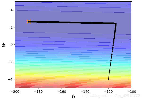
显示结果为：
在这里插入图片描述
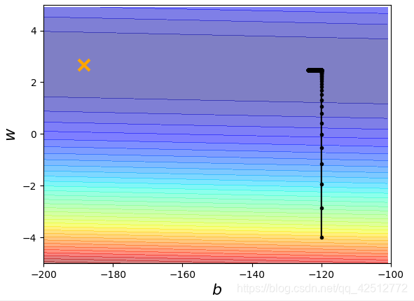
我们发现，在最终得到的结果中，最终回归得到的值离最终的理想状态值相差很大，因此需要调整参数，以达到最终回归出来的值尽可能接近理想值。

x_data = [338., 333., 328., 207., 226., 25., 179., 60., 208., 606.]
y_data = [640., 633., 619., 393., 428., 27., 193., 66., 226., 1591.]
x = np.arange(-200,-100,1)
y = np.arange(-5,5,0.1)
#损失函数
Z = np.zeros((len(x), len(y)))
for i in range(len(x)):
    for j in range(len(y)):
        b = x[i]
        w = y[j]
        Z[j][i] = 0
        for n in range(len(x_data)):
            Z[j][i] = Z[j][i] + (y_data[n] - b - w*x_data[n])**2
        Z[j][i] = Z[j][i] / len(x_data)


def train(lr, iteration):
    # 线性回归原始版
    b = -120
    w = -4

    b_history = [b]
    w_history = [w]

    lr_b = 0
    lr_w = 0

    for i in range(iteration):
        b_grad = 0.0
        w_grad = 0.0
        for n in range(len(x_data)):
            b_grad = b_grad - 2.0 * (y_data[n] - b - w * x_data[n]) * 1.0
            w_grad = w_grad - 2.0 * (y_data[n] - b - w * x_data[n]) * x_data[n]

        lr_b = lr_b + b_grad ** 2
        lr_w = lr_w + w_grad ** 2

        # 更新参数
        b -= lr / np.sqrt(lr_b) * b_grad
        w -= lr / np.sqrt(lr_w) * w_grad

        b_history.append(b)
        w_history.append(w)

    return b_history, w_history

#显示图像
def plot(b_history,w_history):
    plt.contourf(x, y, Z, 50, alpha=0.5, cmap=plt.get_cmap('jet'))
    plt.plot([-188.4], [2.67], 'x', ms=12, markeredgewidth=3, color='orange')
    plt.plot(b_history, w_history, 'o-', ms=3, lw=1.5, color='black')
    plt.xlim(-200, -100)
    plt.ylim(-5, 5)
    plt.xlabel(r'$b$', fontsize=16)
    plt.ylabel(r'$w$', fontsize=16)
    plt.show()


#原始调用lr=0.0000001
iteration = 100000
lr = 1
b_history,w_history=train(lr,iteration)
plot(b_history,w_history)