 TensorFlow神经网络实战


 本文通过实战演示如何使用TensorFlow框架构建神经网络,包括数据预处理、构建模型、训练及预测,以手势数字集为例,深入浅出地解析每个步骤。
6在吴恩达老师的《深度学习》第二课第三周的课程中,提及到了多种深度学习框架,包括caffe/caffe2,CNTK,DL4J,Keras,Lasagne,mxnet,paddlepadle,tensorflow,Theano,Torch等等,虽然Andrew说不特别推荐某种框架,但因其在谷歌多年的经历在之后的练习中终究还是使用tensorflow框架。下面我们跟着达叔的思路一步一步构建深层神经网络。
程序所需的库文件如下
-
import math
-
import numpy
as np
-
import h5py
-
import matplotlib.pyplot
as plt
-
import tensorflow
as tf
-
from tensorflow.python.framework
import ops
-
from tf_utils
import *
-
-
np.random.seed(
1)
tf_utils是吴恩达老师给出的辅助程序,可在这里获取。
一、牛刀小试
1.tensorflow程序执行的步骤
我们先使用tensorflow来对一个简单的损失函数进行计算,Loss公式如下:

-
y_hat = tf.constant(
36, name=
'y_hat')
#创建常数张量,传入数值或者list来填充
-
y = tf.constant(
39, name=
'y')
-
-
loss = tf.Variable((y - y_hat)**
2, name=
'loss')
#创建变量loss
-
-
init = tf.global_variables_initializer()
-
-
with tf.Session()
as session:
-
session.run(init)
-
print(session.run(loss))
测试程序中设y_hat=36,y=39,运行程序结果为:
9
从上述的测试程序中,我们可以了解到tensorflow运行的几个步骤
(1)创建张量tensor(常量或变量);
(2)定义张量之间的运算operations;
(3)初始化*;
(4)创建会话Session*;
(5)在会话中运行操作*。
标*的操作步骤为重要步骤。
2. placeholder的使用
在tf中placeholder是可以稍后赋值的对象,之后在执行session时可通过feed_dict来给placeholder传递值。
-
x = tf.placeholder(tf.int64, name=
'x')
-
with tf.Session()
as sess:
-
print(sess.run(
2 * x, feed_dict = {x:
3}))
-
sess.close()
3.线性函数
我们计算线性函数 Y = WX + b,其中W是(4,3)矩阵,X是(3,1)向量,b是(4,1)向量。
实现代码如下
-
def linear_function():
-
-
np.random.seed(
1)
-
-
X = tf.constant(np.random.randn(
3,
1), name =
"X")
-
W = tf.constant(np.random.randn(
4,
3), name =
"W")
-
b = tf.constant(np.random.randn(
4,
1), name =
"b")
-
Y = tf.add(tf.matmul(W, X), b)
-
-
sess = tf.Session()
-
result = sess.run(Y)
-
sess.close()
-
-
return result
print("Result = " + str(linear_function()))
-
Result = [[
-2.15657382]
-
[
2.95891446]
-
[
-1.08926781]
-
[
-0.84538042]]
4.计算sigmoid
Tensorflow提供了很多神经网络常用的函数,可以直接调用使用,比如sigmoid,softmax,调用方法分别为tf.sigmoid()和tf.softmax,方便开发人员使用。
-
def sigmoid(z):
-
-
x = tf.placeholder(tf.float32, name =
"x")
-
-
sigmoid = tf.sigmoid(x)
-
-
with tf.Session()
as sess:
-
result = sess.run(sigmoid, feed_dict = {x:z})
-
sess.close()
-
-
return result
-
print(
"sigmoid(0) =" + str(sigmoid(
0)))
-
print(
"sigmoid(12) =" + str(sigmoid(
12)))
-
sigmoid(
0) =
0.5
-
sigmoid(
12) =
0.9999938
5.计算cost
cost的计算公式为
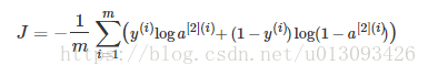
在之前的计算中我们需要使用对i,从1一直算到m,而在Tensorflow框架下,仅需一行代码就可实现这个公式。
-
def cost(logits, labels):
-
-
z = tf.placeholder(tf.float32, name =
"z")
-
y = tf.placeholder(tf.float32, name =
"y")
-
-
cost = tf.nn.sigmoid_cross_entropy_with_logits(logits = z, labels = y)
-
-
sess = tf.Session()
-
-
cost = sess.run(cost, feed_dict = {z:logits, y:labels})
-
-
sess.close()
-
-
return cost
-
logits = sigmoid(np.array([
0.2,
0.4,
0.7,
0.9]))
-
cost = cost(logits, np.array([
0,
0,
1,
1]))
-
print (
"cost = " + str(cost))
cost = [1.0053872 1.0366408 0.41385433 0.39956617]
6."one_hot"转换
对于多分类问题,我们需要将输出值转化为(C, m)矩阵,如下图;
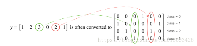
如果使用numpy来实现需要多行代码才能够实现,而在Tensorflow框架下只需要一行代码即可。
-
def one_hot_matrix(labels, C):
-
-
C = tf.constant(value = C, name =
"C")
-
-
one_hot_matrix = tf.one_hot(labels, C, axis =
0)
-
-
sess = tf.Session()
-
-
one_hot = sess.run(one_hot_matrix)
-
-
sess.close()
-
-
return one_hot
-
labels = np.array([
1,
2,
3,
0,
2,
1])
-
one_hot = one_hot_matrix(labels, C =
4)
-
print(
"one_hot = " +
'\n'+ str(one_hot))
-
one_hot = [[
0.
0.
0.
1.
0.
0.]
-
[
1.
0.
0.
0.
0.
1.]
-
[
0.
1.
0.
0.
1.
0.]
-
[
0.
0.
1.
0.
0.
0.]]
二、使用Tensorflow搭建神经网络
看过达叔教程的同学一定会实现神经网络的步骤比较熟悉,下面我们一起跟着达叔的思路用Tensorflow重新搭建一遍深层神经网络。由于之前已经写了多篇关于实现神经网络的文章,在本文中就不再详细描述了。
1.数据处理
达叔在此提供了一个有趣的数据集--手势数字集,如下图。
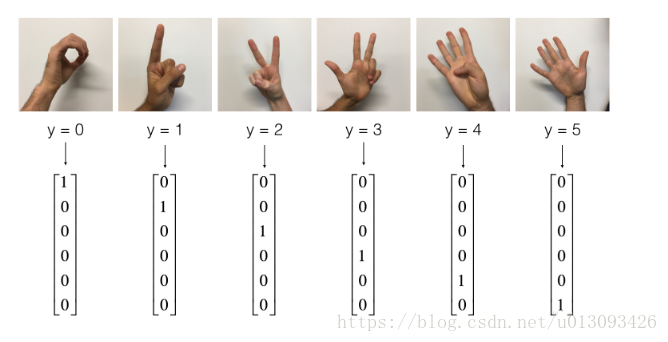
完整数据集点击此处下载。
X_train_orig, Y_train_orig,X_test_orig, Y_test_orig, classes = load_dataset()
-
index =
0
-
plt.imshow(X_train_orig[index])
-
print(
"y=" + str(np.squeeze(Y_train_orig[:,index])))
显示的图片为
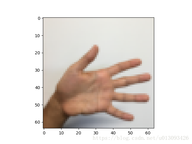
打印的标签是
y= 5
通常导入数据后还要进行flatten、标准化、one-hot处理
-
X_train_flatten = X_train_orig.reshape(X_train_orig.shape[
0],
-1).T
-
X_test_flatten = X_test_orig.reshape(X_test_orig.shape[
0],
-1).T
-
-
X_train = X_train_flatten /
255
-
X_test = X_test_flatten /
255
-
-
Y_train = convert_to_one_hot(Y_train_orig, C =
6)
-
Y_test = convert_to_one_hot(Y_test_orig, C =
6)
-
-
-
print (
"number of training examples = " + str(X_train.shape[
1]))
-
print (
"number of test examples = " + str(X_test.shape[
1]))
-
print (
"X_train shape: " + str(X_train.shape))
-
print (
"Y_train shape: " + str(Y_train.shape))
-
print (
"X_test shape: " + str(X_test.shape))
-
print (
"Y_test shape: " + str(Y_test.shape))
-
number of training examples =
1080
-
number of test examples =
120
-
X_train shape: (
12288,
1080)
-
Y_train shape: (
6,
1080)
-
X_test shape: (
12288,
120)
-
Y_test shape: (
6,
120)
在上述程序中,用到了convert_to_one_hot函数
-
def convert_to_one_hot(Y, C):
-
Y = np.eye(C)[Y.reshape(
-1)].T
-
return Y
很巧妙的使用了矩阵的特性来实现one-hot变换。提示:np.array((3,4))[1] -> 输出为该矩阵的第2行
2.创建placeholders
为了后续传入训练数据,我们需要先创建X和Y的占位符。
-
def create_placeholder(n_x, n_y):
-
-
X = tf.placeholder(tf.float32, shape = [n_x,
None])
-
-
Y = tf.placeholder(tf.float32, shape = [n_y,
None])
-
-
return X, Y
-
X, Y = create_placeholder(
12288,
6)
-
print(
"X = " + str(X))
-
print(
"Y = " + str(Y))
-
X = Tensor(
"Placeholder:0", shape=(
12288, ?), dtype=float32)
-
Y = Tensor(
"Placeholder_1:0", shape=(
6, ?), dtype=float32)
我们使用Tensorflow来初始化参数W和b
-
def initialize_parameters():
-
-
tf.set_random_seed(
1)
-
-
W1 = tf.get_variable(
"W1", [
25,
12288], initializer = tf.contrib.layers.xavier_initializer(seed =
1))
-
b1 = tf.get_variable(
"b1", [
25,
1], initializer = tf.zeros_initializer())
-
W2 = tf.get_variable(
"W2", [
12,
25], initializer = tf.contrib.layers.xavier_initializer(seed =
1))
-
b2 = tf.get_variable(
"b2", [
12,
1], initializer = tf.zeros_initializer())
-
W3 = tf.get_variable(
"W3", [
6,
12], initializer = tf.contrib.layers.xavier_initializer(seed =
1))
-
b3 = tf.get_variable(
"b3", [
6,
1], initializer = tf.zeros_initializer())
-
-
parameters = {
"W1" : W1,
-
"b1" : b1,
-
"W2" : W2,
-
"b2" : b2,
-
"W3" : W3,
-
"b3" : b3}
-
-
return parameters
-
with tf.Session()
as sess:
-
parameters = initialize_parameters()
-
-
print(
"W1 = " + str(parameters[
"W1"]))
-
print(
"b1 = " + str(parameters[
"b1"]))
-
print(
"W2 = " + str(parameters[
"W2"]))
-
print(
"b2 = " + str(parameters[
"b2"]))
-
W1 = <tf.Variable
'W1:0' shape=(
25,
12288) dtype=float32_ref>
-
b1 = <tf.Variable
'b1:0' shape=(
25,
1) dtype=float32_ref>
-
W2 = <tf.Variable
'W2:0' shape=(
12,
25) dtype=float32_ref>
-
b2 = <tf.Variable
'b2:0' shape=(
12,
1) dtype=float32_ref>
4.前向传播
-
def forward_propagation(X, parameters):
-
-
W1 = parameters[
'W1']
-
b1 = parameters[
'b1']
-
W2 = parameters[
'W2']
-
b2 = parameters[
'b2']
-
W3 = parameters[
'W3']
-
b3 = parameters[
'b3']
-
-
Z1 = tf.add(tf.matmul(W1, X), b1)
-
A1 = tf.nn.relu(Z1)
-
Z2 = tf.add(tf.matmul(W2, A1), b2)
-
A2 = tf.nn.relu(Z2)
-
Z3 = tf.add(tf.matmul(W3, A2), b3)
-
-
return Z3
-
tf.reset_default_graph()
-
with tf.Session()
as sess:
-
X, Y = create_placeholder(
12288,
6)
-
parameters = initialize_parameters()
-
Z3 = forward_propagation(X, parameters)
-
-
print(
"Z3 =", Z3)
Z3 = Tensor("Add_2:0", shape=(6, ?), dtype=float32)
5.计算cost
-
def compute_cost(Z3, Y):
-
-
logits = tf.transpose(Z3)
-
labels = tf.transpose(Y)
-
-
cost = tf.reduce_mean(tf.nn.softmax_cross_entropy_with_logits(logits = logits, labels = labels))
-
-
return cost
-
tf.reset_default_graph()
-
with tf.Session()
as sess:
-
X, Y = create_placeholder(
12288,
6)
-
parameters = initialize_parameters()
-
Z3 = forward_propagation(X, parameters)
-
cost = compute_cost(Z3, Y)
-
-
print(
"cost =", cost)
cost = Tensor("Mean:0", shape=(), dtype=float32)
6.反向传播及参数更新
由于使用深度学习框架,我们可以把反向传播和参数更新浓缩成一行代码,且很容易整合到模型中。在计算完cost函数后,我们需要创建一个“optimizer”对象,以便执行给定梯度下降的方法和学习率
optimizer = tf.train.GradientDescentOptimizer(learning_rate = learning_rate).minimize(cost)
使该优化生效,在sess.run中需要做下述处理。
_, c = sess.run([optimizer, cost], feed_dict = {X: minibatch_X, Y:minibatch_Y})
注:"_"为丢弃变量的标识符,在此我们只需sess.run()返回的cost值因此使用c来接收返回值,optimizer的值无需使用因此使用"_"来接收。
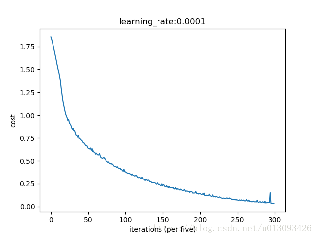
7.构建模型
现在我们将上述的函数整合到一起构建一个基于Tensorflow的神经网络模型。
-
def model(X_train, Y_train, X_test, Y_test, learning_rate = 0.0001,
-
num_epochs = 1500, minibatch_size = 32, print_cost = True):
-
-
ops.reset_default_graph()
-
tf.set_random_seed(
1)
-
seed =
3
-
(n_x, m) = X_train.shape
-
n_y = Y_train.shape[
0]
-
costs = []
-
-
X, Y = create_placeholder(n_x, n_y)
-
parameters = initialize_parameters()
-
Z3 = forward_propagation(X, parameters)
-
cost = compute_cost(Z3, Y)
-
optimizer = tf.train.AdamOptimizer(learning_rate = learning_rate).minimize(cost)
-
-
init = tf.global_variables_initializer()
-
with tf.Session()
as sess:
-
sess.run(init)
-
for epoch
in range(num_epochs):
-
epoch_cost =
0.
-
num_minibatches = int(m / minibatch_size)
-
seed = seed +
1
-
minibatches = random_mini_batches(X_train, Y_train, minibatch_size, seed)
-
-
for minibatch
in minibatches:
-
(minibatch_X, minibatch_Y) = minibatch
-
_ , minibatch_cost = sess.run([optimizer, cost], feed_dict = {X: minibatch_X, Y:minibatch_Y})
-
epoch_cost += minibatch_cost / num_minibatches
-
-
if print_cost
and epoch %
100 ==
0:
-
print(
"Cost after epoch %i: %f" %(epoch, epoch_cost))
-
-
if print_cost
and epoch %
5 ==
0:
-
costs.append(epoch_cost)
-
-
plt.plot(np.squeeze(costs))
-
plt.xlabel(
"iterations (per five)")
-
plt.ylabel(
"cost")
-
plt.title(
"learning_rate:" + str(learning_rate))
-
plt.show()
-
-
parameters = sess.run(parameters)
-
print(
"Parameters have been trained!")
-
-
correct_prediction = tf.equal(tf.argmax(Z3), tf.argmax(Y))
-
-
accuracy = tf.reduce_mean(tf.cast(correct_prediction,
"float"))
-
-
print(
"Train Accuray:", accuracy.eval({X: X_train, Y: Y_train}))
-
print(
"Test Accuray:", accuracy.eval({X: X_test, Y: Y_test}))
-
-
return parameters
程序在执行时需要一定时间,大家注意下如果在epoch 100时cost值不是1.016458,可以停止程序查找问题不必要浪费时间。
parameters = model(X_train, Y_train, X_test, Y_test)
-
Cost after epoch
0:
1.855702
-
Cost after epoch
100:
1.016458
-
Cost after epoch
200:
0.733102
-
Cost after epoch
300:
0.572938
-
Cost after epoch
400:
0.468799
-
Cost after epoch
500:
0.380979
-
Cost after epoch
600:
0.313819
-
Cost after epoch
700:
0.254258
-
Cost after epoch
800:
0.203795
-
Cost after epoch
900:
0.166410
-
Cost after epoch
1000:
0.141497
-
Cost after epoch
1100:
0.107579
-
Cost after epoch
1200:
0.086229
-
Cost after epoch
1300:
0.059415
-
Cost after epoch
1400:
0.052237
-
Parameters have been trained!
-
Train Accuray:
0.9990741
-
Test Accuray:
0.71666664
三、图片预测
在完成了模型搭建的任务之后,我们来测试一下自己的手势图片,如下图。

我们将该图片进行一些处理转化成64*64*3格式以便测试。
-
my_image =
"myfigure.jpg"
-
fname =
"images\\" + my_image
-
-
image = np.array(ndimage.imread(fname, flatten=
False))
-
my_image = scipy.misc.imresize(image, size=(
64,
64)).reshape((
1,
64*
64*
3)).T
-
my_image_prediction = predict(my_image, parameters)
-
-
plt.imshow(image)
-
print(
"your algorithm predicts : y=" + str(np.squeeze(my_image_prediction)))
your algorithm predicts : y=4
四、总结
1.Tensorflow是深度学习的框架,其最重要的两个类是Tensor和Operaters
2.在框架下编程时要注意在第一节中的步骤
3.graph可以多次执行
4.反向传播和优化过程是框架自动完成


 1124
1124

 被折叠的 条评论
为什么被折叠?
被折叠的 条评论
为什么被折叠?
 到【灌水乐园】发言


