LLMs-from-scratch（第4章：从零开始实现GPT模型以生成文本）

最新推荐文章于 2025-11-23 21:54:14 发布

原创最新推荐文章于 2025-11-23 21:54:14 发布 · 1.3k 阅读

30 ·

CC 4.0 BY-SA版权

文章标签：

#gpt #llm

大模型结构专栏收录该内容

37 篇文章

订阅专栏

代码链接：https://github.com/rasbt/LLMs-from-scratch/ch04/01_main-chapter-code/ch04.ipynb

Sebastian Raschka 著作《从零开始构建大型语言模型》的补充代码

代码仓库：https://github.com/rasbt/LLMs-from-scratch

第4章：从零开始实现GPT模型以生成文本

from importlib.metadata import version

print("matplotlib version:", version("matplotlib"))
print("torch version:", version("torch"))
print("tiktoken version:", version("tiktoken"))

matplotlib version: 3.10.7
torch version: 2.5.1+cu124
tiktoken version: 0.12.0

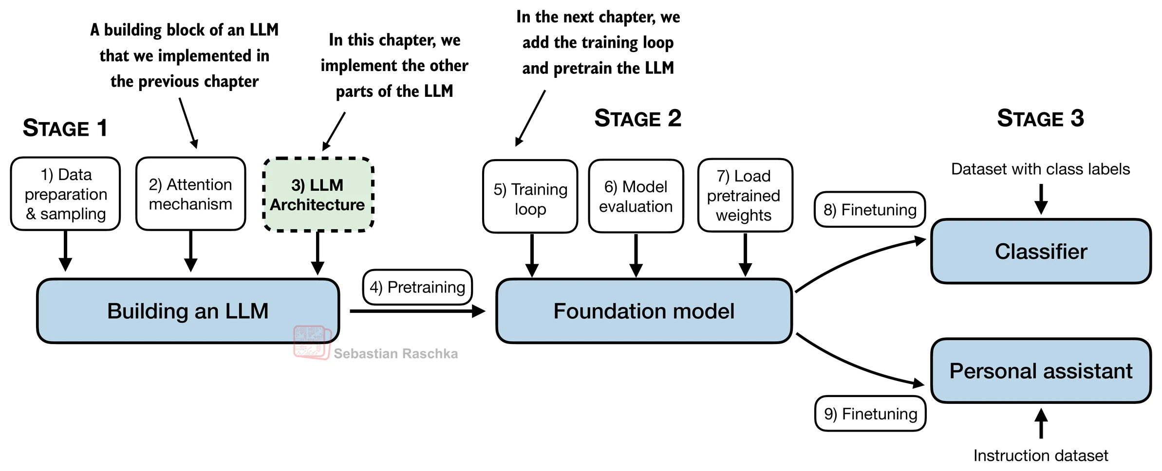
在本章中，我们实现了一个类似GPT的LLM架构；下一章将专注于训练这个LLM

4.1 编写LLM架构代码

第1章讨论了像GPT和Llama这样的模型，它们按顺序生成单词，并基于原始transformer架构的解码器部分
因此，这些LLM通常被称为"类解码器"LLM
与传统的深度学习模型相比，LLM更大，主要是由于它们拥有大量的参数，而不是代码量
我们将看到LLM架构中有许多重复的元素

在前面的章节中，我们为了便于说明，使用了较小的嵌入维度来处理token输入和输出，确保它们能在单页上显示
在本章中，我们考虑类似于小型GPT-2模型的嵌入和模型大小
我们将专门编写最小GPT-2模型（1.24亿参数）的架构，如Radford等人的《语言模型是无监督多任务学习器》中所述（注意初始报告将其列为1.17亿参数，但后来在模型权重仓库中进行了更正）
第6章将展示如何将预训练权重加载到我们的实现中，这将与3.45亿、7.62亿和15.42亿参数的模型大小兼容
1.24亿参数GPT-2模型的配置详情包括：

GPT_CONFIG_124M = {
    "vocab_size": 50257,    # 词汇表大小
    "context_length": 1024, # 上下文长度
    "emb_dim": 768,         # 嵌入维度
    "n_heads": 12,          # 注意力头数量
    "n_layers": 12,         # 层数
    "drop_rate": 0.1,       # Dropout率
    "qkv_bias": False       # 查询-键-值偏置
}

我们使用简短的变量名以避免后续代码行过长
"vocab_size"表示词汇表大小为50,257个单词，由第2章讨论的BPE分词器支持
"context_length"表示模型的最大输入token数量，由第2章涵盖的位置嵌入启用
"emb_dim"是token输入的嵌入大小，将每个输入token转换为768维向量
"n_heads"是第3章实现的多头注意力机制中的注意力头数量
"n_layers"是模型内transformer块的数量，我们将在接下来的部分中实现
"drop_rate"是dropout机制的强度，在第3章中讨论；0.1意味着在训练期间丢弃10%的隐藏单元以减轻过拟合
"qkv_bias"决定多头注意力机制（来自第3章）中的Linear层在计算查询(Q)、键(K)和值(V)张量时是否应包含偏置向量；我们将禁用此选项，这是现代LLM的标准做法；但是，当我们在第5章将预训练的GPT-2权重从OpenAI加载到我们的重新实现中时，我们将重新讨论这一点

import torch
import torch.nn as nn

class DummyGPTModel(nn.Module):
    def __init__(self, cfg):
        super().__init__()
        self.tok_emb = nn.Embedding(cfg["vocab_size"], cfg["emb_dim"])
        self.pos_emb = nn.Embedding(cfg["context_length"], cfg["emb_dim"])
        self.drop_emb = nn.Dropout(cfg["drop_rate"])
        
        # 使用TransformerBlock的占位符
        self.trf_blocks = nn.Sequential(
            *[DummyTransformerBlock(cfg) for _ in range(cfg["n_layers"])])
        
        # 使用LayerNorm的占位符
        self.final_norm = DummyLayerNorm(cfg["emb_dim"])
        self.out_head = nn.Linear(
            cfg["emb_dim"], cfg["vocab_size"], bias=False
        )

    def forward(self, in_idx):
        batch_size, seq_len = in_idx.shape
        tok_embeds = self.tok_emb(in_idx)
        pos_embeds = self.pos_emb(torch.arange(seq_len, device=in_idx.device))
        x = tok_embeds + pos_embeds
        x = self.drop_emb(x)
        x = self.trf_blocks(x)
        x = self.final_norm(x)
        logits = self.out_head(x)
        return logits

class DummyTransformerBlock(nn.Module):
    def __init__(self, cfg):
        super().__init__()
        # 一个简单的占位符

    def forward(self, x):
        # 这个块什么都不做，只是返回输入
        return x

class DummyLayerNorm(nn.Module):
    def __init__(self, normalized_shape, eps=1e-5):
        super().__init__()
        # 这里的参数只是为了模拟LayerNorm接口

    def forward(self, x):
        # 这个层什么都不做，只是返回输入
        return x

import tiktoken

tokenizer = tiktoken.get_encoding("gpt2")

batch = []

txt1 = "Every effort moves you"
txt2 = "Every day holds a"

batch.append(torch.tensor(tokenizer.encode(txt1)))
batch.append(torch.tensor(tokenizer.encode(txt2)))
batch = torch.stack(batch, dim=0)
print(batch)

tensor([[6109, 3626, 6100,  345],
        [6109, 1110, 6622,  257]])

torch.manual_seed(123)
model = DummyGPTModel(GPT_CONFIG_124M)

logits = model(batch)
print("Output shape:", logits.shape)
print(logits)

Output shape: torch.Size([2, 4, 50257])
tensor([[[-0.9289,  0.2748, -0.7557,  ..., -1.6070,  0.2702, -0.5888],
         [-0.4476,  0.1726,  0.5354,  ..., -0.3932,  1.5285,  0.8557],
         [ 0.5680,  1.6053, -0.2155,  ...,  1.1624,  0.1380,  0.7425],
         [ 0.0447,  2.4787, -0.8843,  ...,  1.3219, -0.0864, -0.5856]],

        [[-1.5474, -0.0542, -1.0571,  ..., -1.8061, -0.4494, -0.6747],
         [-0.8422,  0.8243, -0.1098,  ..., -0.1434,  0.2079,  1.2046],
         [ 0.1355,  1.1858, -0.1453,  ...,  0.0869, -0.1590,  0.1552],
         [ 0.1666, -0.8138,  0.2307,  ...,  2.5035, -0.3055, -0.3083]]],
       grad_fn=<UnsafeViewBackward0>)

注意

如果您在Windows或Linux上运行此代码，上述结果值可能如下所示：

Output shape: torch.Size([2, 4, 50257])
tensor([[[-0.9289,  0.2748, -0.7557,  ..., -1.6070,  0.2702, -0.5888],
         [-0.4476,  0.1726,  0.5354,  ..., -0.3932,  1.5285,  0.8557],
         [ 0.5680,  1.6053, -0.2155,  ...,  1.1624,  0.1380,  0.7425],
         [ 0.0447,  2.4787, -0.8843,  ...,  1.3219, -0.0864, -0.5856]],

        [[-1.5474, -0.0542, -1.0571,  ..., -1.8061, -0.4494, -0.6747],
         [-0.8422,  0.8243, -0.1098,  ..., -0.1434,  0.2079,  1.2046],
         [ 0.1355,  1.1858, -0.1453,  ...,  0.0869, -0.1590,  0.1552],
         [ 0.1666, -0.8138,  0.2307,  ...,  2.5035, -0.3055, -0.3083]]],
       grad_fn=<UnsafeViewBackward0>)

由于这些只是随机数字，这不是令人担心的原因，您可以继续本章的其余部分而不会有问题
造成这种差异的一个可能原因是nn.Dropout在不同操作系统上的行为不同，这取决于PyTorch的编译方式，如PyTorch问题跟踪器上的讨论

4.2 使用层归一化来归一化激活

层归一化，也称为LayerNorm（Ba等人，2016），将神经网络层的激活以均值0为中心，并将其方差归一化为1
这稳定了训练并能够更快地收敛到有效权重
层归一化在transformer块内的多头注意力模块之前和之后都会应用，我们稍后将实现；它也在最终输出层之前应用

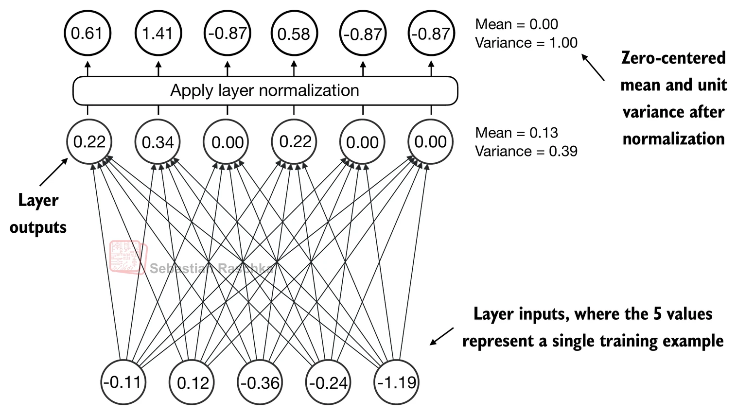
让我们通过将一个小输入样本传递给一个简单的神经网络层来看看层归一化是如何工作的：

torch.manual_seed(123)

# 创建2个训练样本，每个有5个维度（特征）
batch_example = torch.randn(2, 5) 

layer = nn.Sequential(nn.Linear(5, 6), nn.ReLU())
out = layer(batch_example)
print(out)

tensor([[0.2260, 0.3470, 0.0000, 0.2216, 0.0000, 0.0000],
        [0.2133, 0.2394, 0.0000, 0.5198, 0.3297, 0.0000]],
       grad_fn=<ReluBackward0>)

让我们计算上述2个输入的均值和方差：

mean = out.mean(dim=-1, keepdim=True)
var = out.var(dim=-1, keepdim=True)

print("均值:\n", mean)
print("方差:\n", var)

Mean:
 tensor([[0.1324],
        [0.2170]], grad_fn=<MeanBackward1>)
Variance:
 tensor([[0.0231],
        [0.0398]], grad_fn=<VarBackward0>)

归一化独立应用于两个输入（行）中的每一个；使用dim=-1在最后一个维度（在这种情况下是特征维度）而不是行维度上应用计算

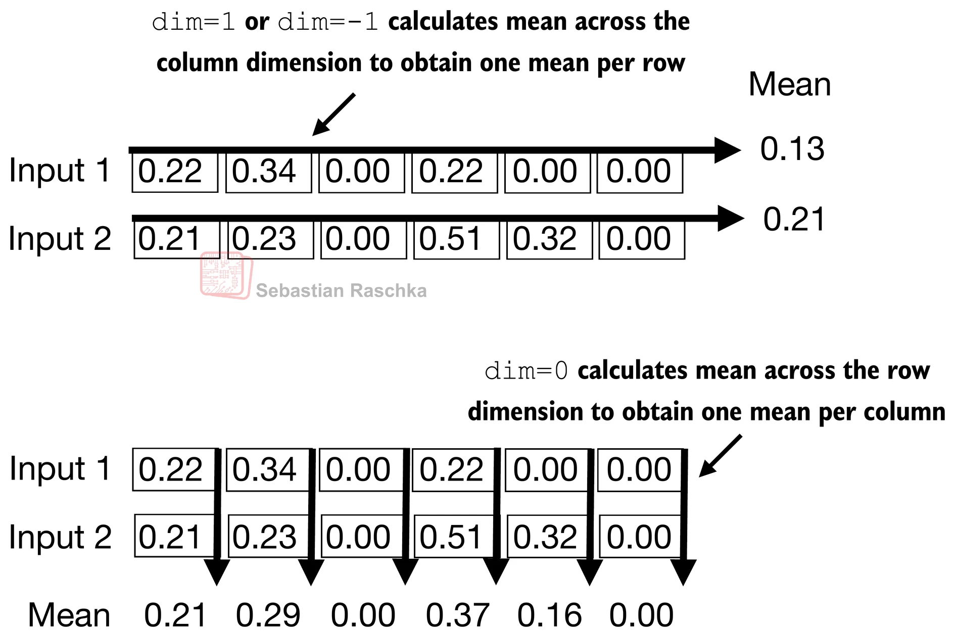
减去均值并除以方差的平方根（标准差）将输入居中，使其在列（特征）维度上具有0的均值和1的方差：

out_norm = (out - mean) / torch.sqrt(var)
print("归一化后的层输出:\n", out_norm)

mean = out_norm.mean(dim=-1, keepdim=True)
var = out_norm.var(dim=-1, keepdim=True)
print("归一化后的均值:\n", mean)
print("归一化后的方差:\n", var)

Normalized layer outputs:
 tensor([[ 0.6159,  1.4126, -0.8719,  0.5872, -0.8719, -0.8719],
        [-0.0189,  0.1121, -1.0876,  1.5173,  0.5647, -1.0876]],
       grad_fn=<DivBackward0>)
Mean:
 tensor([[9.9341e-09],
        [0.0000e+00]], grad_fn=<MeanBackward1>)
Variance:
 tensor([[1.0000],
        [1.0000]], grad_fn=<VarBackward0>)

每个输入都以0为中心，具有1的单位方差；为了提高可读性，我们可以禁用PyTorch的科学记数法：

torch.set_printoptions(sci_mode=False)
print("Mean:\n", mean)
print("Variance:\n", var)

Mean:
 tensor([[    0.0000],
        [    0.0000]], grad_fn=<MeanBackward1>)
Variance:
 tensor([[1.0000],
        [1.0000]], grad_fn=<VarBackward0>)

上面，我们对每个输入的特征进行了归一化
现在，使用相同的思想，我们可以实现一个LayerNorm类：

class LayerNorm(nn.Module):
    def __init__(self, emb_dim):
        super().__init__()
        self.eps = 1e-5
        self.scale = nn.Parameter(torch.ones(emb_dim))
        self.shift = nn.Parameter(torch.zeros(emb_dim))

    def forward(self, x):
        mean = x.mean(dim=-1, keepdim=True)
        var = x.var(dim=-1, keepdim=True, unbiased=False)
        norm_x = (x - mean) / torch.sqrt(var + self.eps)
        return self.scale * norm_x + self.shift

缩放和偏移

注意，除了通过减去均值和除以方差来执行归一化之外，我们还添加了两个可训练参数：scale和shift参数
初始的scale（乘以1）和shift（加0）值没有任何效果；然而，scale和shift是可训练参数，如果确定这样做能提高模型在训练任务上的性能，LLM会在训练期间自动调整这些参数
这允许模型学习最适合其处理数据的适当缩放和偏移
注意我们还在计算方差的平方根之前添加了一个较小的值（eps）；这是为了避免在方差为0时出现除零错误

有偏方差

在上面的方差计算中，设置unbiased=False意味着使用公式 $\frac{\sum_i (x_i - \bar{x})^2}{n}$ 来计算方差，其中n是样本大小（这里是特征或列的数量）；这个公式不包括贝塞尔校正（在分母中使用n-1），因此提供了方差的有偏估计
对于LLM，其中嵌入维度n非常大，使用n和n-1之间的差异是可以忽略的
然而，GPT-2在归一化层中使用有偏方差进行训练，这就是为什么我们也采用这种设置以与我们将在后续章节中加载的预训练权重兼容的原因
现在让我们在实践中尝试LayerNorm：

ln = LayerNorm(emb_dim=5)
out_ln = ln(batch_example)

mean = out_ln.mean(dim=-1, keepdim=True)
var = out_ln.var(dim=-1, unbiased=False, keepdim=True)

print("LayerNorm后的均值:\n", mean)
print("LayerNorm后的方差:\n", var)

Mean:
 tensor([[    -0.0000],
        [     0.0000]], grad_fn=<MeanBackward1>)
Variance:
 tensor([[1.0000],
        [1.0000]], grad_fn=<VarBackward0>)

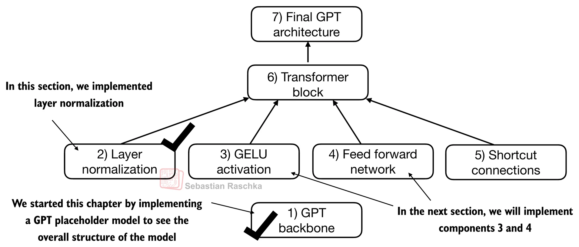
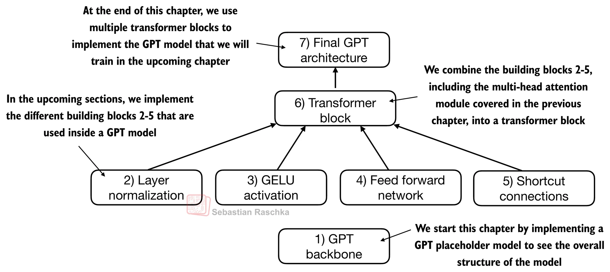
4.3 使用GELU激活函数实现前馈网络

在本节中，我们实现一个小型神经网络子模块，它作为LLM中transformer块的一部分使用
我们从激活函数开始
在深度学习中，ReLU（修正线性单元）激活函数由于其简单性和在各种神经网络架构中的有效性而被广泛使用
在LLM中，除了传统的ReLU之外，还使用各种其他类型的激活函数；两个显著的例子是GELU（高斯误差线性单元）和SwiGLU（Swish门控线性单元）
GELU和SwiGLU是更复杂、更平滑的激活函数，分别结合了高斯和sigmoid门控线性单元，与ReLU更简单的分段线性函数相比，为深度学习模型提供了更好的性能
GELU（Hendrycks和Gimpel 2016）可以通过几种方式实现；精确版本定义为GELU(x)=x⋅Φ(x)，其中Φ(x)是标准高斯分布的累积分布函数。
在实践中，通常实现一个计算成本更低的近似： $\text{GELU}(x) \approx 0.5 \cdot x \cdot \left(1 + \tanh\left[\sqrt{\frac{2}{\pi}} \cdot \left(x + 0.044715 \cdot x^3\right)\right]\right)$ （原始的GPT-2模型也是用这个近似训练的）

class GELU(nn.Module):
    def __init__(self):
        super().__init__()

    def forward(self, x):
        return 0.5 * x * (1 + torch.tanh(
            torch.sqrt(torch.tensor(2.0 / torch.pi)) * 
            (x + 0.044715 * torch.pow(x, 3))
        ))

import matplotlib.pyplot as plt

gelu, relu = GELU(), nn.ReLU()

# 一些样本数据
x = torch.linspace(-3, 3, 100)
y_gelu, y_relu = gelu(x), relu(x)


plt.figure(figsize=(8, 3))
for i, (y, label) in enumerate(zip([y_gelu, y_relu], ["GELU", "ReLU"]), 1):
    plt.subplot(1, 2, i)
    plt.plot(x, y)
    plt.title(f"{label} activation function")
    plt.xlabel("x")
    plt.ylabel(f"{label}(x)")
    plt.grid(True)

plt.tight_layout()
plt.show()

在这里插入图片描述

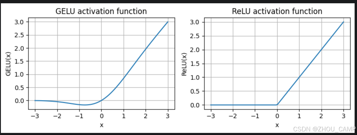
如我们所见，ReLU是一个分段线性函数，如果输入为正则直接输出输入；否则输出零
GELU是一个平滑的非线性函数，近似于ReLU，但对于负值具有非零梯度（除了大约-0.75处）
接下来，让我们实现小型神经网络模块FeedForward，我们稍后将在LLM的transformer块中使用它：

class FeedForward(nn.Module):
    def __init__(self, cfg):
        super().__init__()
        self.layers = nn.Sequential(
            nn.Linear(cfg["emb_dim"], 4 * cfg["emb_dim"]),
            GELU(),
            nn.Linear(4 * cfg["emb_dim"], cfg["emb_dim"]),
        )

    def forward(self, x):
        return self.layers(x)

print(GPT_CONFIG_124M["emb_dim"])

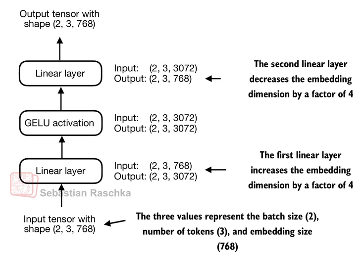
ffn = FeedForward(GPT_CONFIG_124M)

# 输入形状: [batch_size, num_token, emb_size]
x = torch.rand(2, 3, 768) 
out = ffn(x)
print(out.shape)

torch.Size([2, 3, 768])

4.4 添加快捷连接

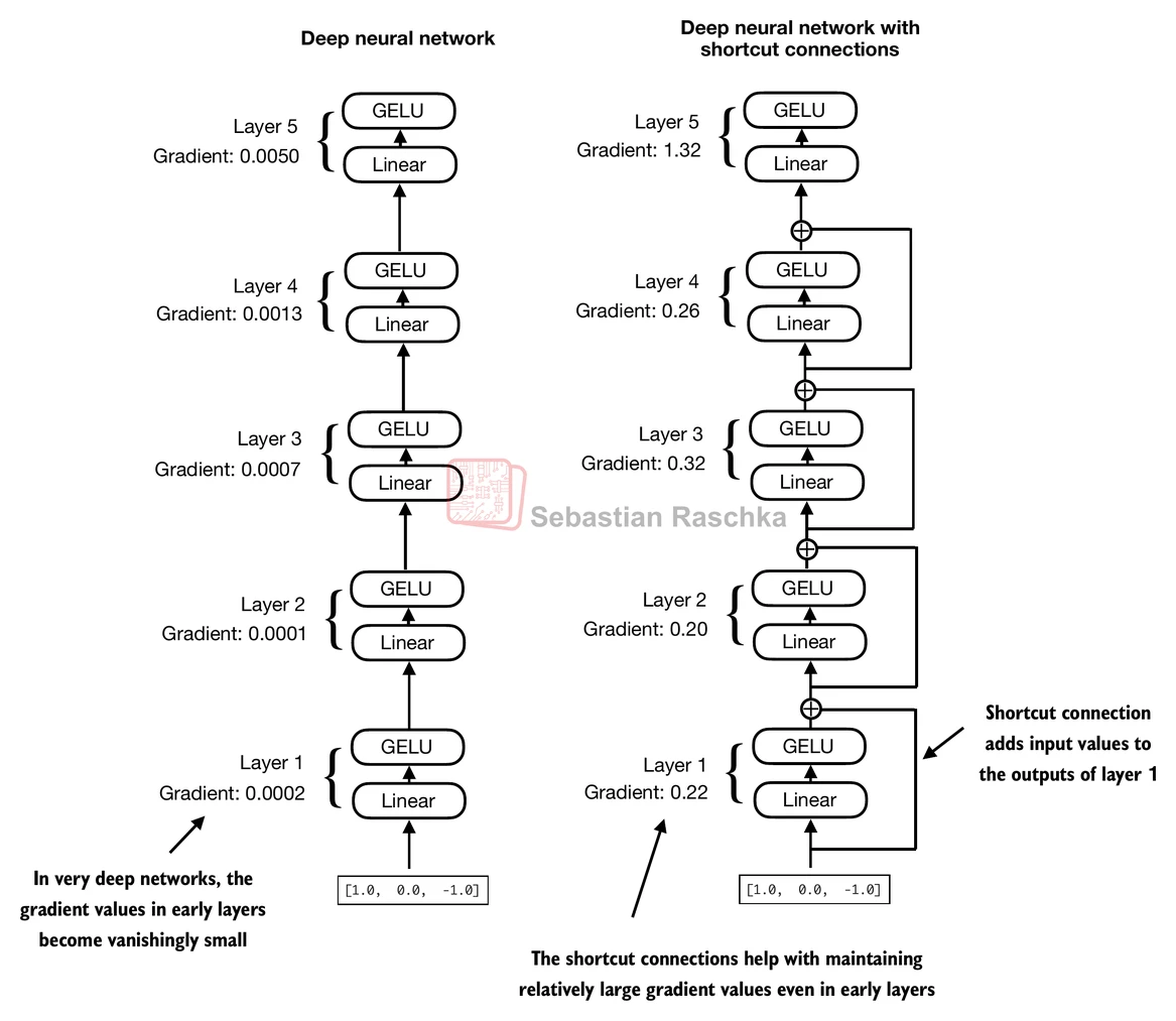
接下来，让我们讨论快捷连接背后的概念，也称为跳跃连接或残差连接
最初，快捷连接是在计算机视觉的深度网络（残差网络）中提出的，用于缓解梯度消失问题
快捷连接为梯度在网络中流动创建了一条替代的更短路径
这是通过将一层的输出添加到后面一层的输出来实现的，通常跳过中间的一层或多层
让我们用一个小型示例网络来说明这个想法：

在代码中，它看起来像这样：

class ExampleDeepNeuralNetwork(nn.Module):
    def __init__(self, layer_sizes, use_shortcut):
        super().__init__()
        self.use_shortcut = use_shortcut
        self.layers = nn.ModuleList([
            nn.Sequential(nn.Linear(layer_sizes[0], layer_sizes[1]), GELU()),
            nn.Sequential(nn.Linear(layer_sizes[1], layer_sizes[2]), GELU()),
            nn.Sequential(nn.Linear(layer_sizes[2], layer_sizes[3]), GELU()),
            nn.Sequential(nn.Linear(layer_sizes[3], layer_sizes[4]), GELU()),
            nn.Sequential(nn.Linear(layer_sizes[4], layer_sizes[5]), GELU())
        ])

    def forward(self, x):
        for layer in self.layers:
            # 计算当前层的输出
            layer_output = layer(x)
            # 检查是否可以应用快捷连接
            if self.use_shortcut and x.shape == layer_output.shape:
                x = x + layer_output
            else:
                x = layer_output
        return x


def print_gradients(model, x):
    # 前向传播
    output = model(x)
    target = torch.tensor([[0.]])

    # 基于目标和输出的接近程度计算损失
    loss = nn.MSELoss()
    loss = loss(output, target)
    
    # 反向传播计算梯度
    loss.backward()

    for name, param in model.named_parameters():

    if 'weight' in name:
        # 打印权重的平均绝对梯度
        print(f"{name} has gradient mean of {param.grad.abs().mean().item()}")


- 让我们首先打印**没有**快捷连接的梯度值：


```python
layer_sizes = [3, 3, 3, 3, 3, 1]  

sample_input = torch.tensor([[1., 0., -1.]])

torch.manual_seed(123)
model_without_shortcut = ExampleDeepNeuralNetwork(
    layer_sizes, use_shortcut=False
)
print_gradients(model_without_shortcut, sample_input)

layers.0.0.weight has gradient mean of 0.00020173587836325169
layers.1.0.weight has gradient mean of 0.0001201116101583466
layers.2.0.weight has gradient mean of 0.0007152041653171182
layers.3.0.weight has gradient mean of 0.001398873864673078
layers.4.0.weight has gradient mean of 0.005049646366387606

接下来，让我们打印有快捷连接的梯度值：

torch.manual_seed(123)
model_with_shortcut = ExampleDeepNeuralNetwork(
    layer_sizes, use_shortcut=True
)
print_gradients(model_with_shortcut, sample_input)

layers.0.0.weight has gradient mean of 0.22169792652130127
layers.1.0.weight has gradient mean of 0.20694106817245483
layers.2.0.weight has gradient mean of 0.32896995544433594
layers.3.0.weight has gradient mean of 0.2665732502937317
layers.4.0.weight has gradient mean of 1.3258541822433472

如我们从上面的输出中可以看到，快捷连接防止了梯度在早期层（朝向layer.0）中消失
接下来当我们实现transformer块时，我们将使用这个快捷连接的概念

4.5 在transformer块中连接注意力和线性层

在本节中，我们现在将之前的概念组合成所谓的transformer块
transformer块将前一章的因果多头注意力模块与线性层、我们在前面章节中实现的前馈神经网络结合起来
此外，transformer块还使用dropout和快捷连接

class MultiHeadAttention(nn.Module):
    def __init__(self, d_in, d_out, context_length, dropout, num_heads, qkv_bias=False):
        super().__init__()
        assert (d_out % num_heads == 0), \
            "d_out must be divisible by num_heads"

        self.d_out = d_out
        self.num_heads = num_heads
        self.head_dim = d_out // num_heads # 减少投影维度以匹配所需的输出维度 

        self.W_query = nn.Linear(d_in, d_out, bias=qkv_bias)
        self.W_key = nn.Linear(d_in, d_out, bias=qkv_bias)
        self.W_value = nn.Linear(d_in, d_out, bias=qkv_bias)
        self.out_proj = nn.Linear(d_out, d_out)  # 用于组合头输出的线性层
        self.dropout = nn.Dropout(dropout)
        self.register_buffer(
            "mask",
            torch.triu(torch.ones(context_length, context_length),
                       diagonal=1)
        )

    def forward(self, x):
        b, num_tokens, d_in = x.shape
        # 如在`CausalAttention`中，对于`num_tokens`超过`context_length`的输入，
        # 这将在下面的掩码创建中导致错误。
        # 在实践中，这不是问题，因为LLM（第4-7章）确保输入
        # 在到达此前向方法之前不会超过`context_length`。

        keys = self.W_key(x) # 形状: (b, num_tokens, d_out)
        queries = self.W_query(x)
        values = self.W_value(x)

        # 我们通过添加`num_heads`维度隐式地分割矩阵
        # 展开最后一个维度: (b, num_tokens, d_out) -> (b, num_tokens, num_heads, head_dim)
        keys = keys.view(b, num_tokens, self.num_heads, self.head_dim) 
        values = values.view(b, num_tokens, self.num_heads, self.head_dim)
        queries = queries.view(b, num_tokens, self.num_heads, self.head_dim)

        # 转置: (b, num_tokens, num_heads, head_dim) -> (b, num_heads, num_tokens, head_dim)
        keys = keys.transpose(1, 2)
        queries = queries.transpose(1, 2)
        values = values.transpose(1, 2)

        # 使用因果掩码计算缩放点积注意力（也称为自注意力）
        attn_scores = queries @ keys.transpose(2, 3)  # 每个头的点积

        # 原始掩码截断到token数量并转换为布尔值
        mask_bool = self.mask.bool()[:num_tokens, :num_tokens]

        # 使用掩码填充注意力分数
        attn_scores.masked_fill_(mask_bool, -torch.inf)
        
        attn_weights = torch.softmax(attn_scores / keys.shape[-1]**0.5, dim=-1)
        attn_weights = self.dropout(attn_weights)

        # 形状: (b, num_tokens, num_heads, head_dim)
        context_vec = (attn_weights @ values).transpose(1, 2) 
        
        # 组合头，其中self.d_out = self.num_heads * self.head_dim
        context_vec = context_vec.contiguous().view(b, num_tokens, self.d_out)
        context_vec = self.out_proj(context_vec) # 可选的投影

        return context_vec

class TransformerBlock(nn.Module):
    def __init__(self, cfg):
        super().__init__()
        self.att = MultiHeadAttention(
            d_in=cfg["emb_dim"],
            d_out=cfg["emb_dim"],
            context_length=cfg["context_length"],
            num_heads=cfg["n_heads"], 
            dropout=cfg["drop_rate"],
            qkv_bias=cfg["qkv_bias"])
        self.ff = FeedForward(cfg)
        self.norm1 = LayerNorm(cfg["emb_dim"])
        self.norm2 = LayerNorm(cfg["emb_dim"])
        self.drop_shortcut = nn.Dropout(cfg["drop_rate"])

    def forward(self, x):
        # 注意力块的快捷连接
        shortcut = x
        x = self.norm1(x)
        x = self.att(x)  # 形状 [batch_size, num_tokens, emb_size]
        x = self.drop_shortcut(x)
        x = x + shortcut  # 将原始输入加回

        # 前馈块的快捷连接
        shortcut = x
        x = self.norm2(x)
        x = self.ff(x)
        x = self.drop_shortcut(x)
        x = x + shortcut  # 将原始输入加回

        return x

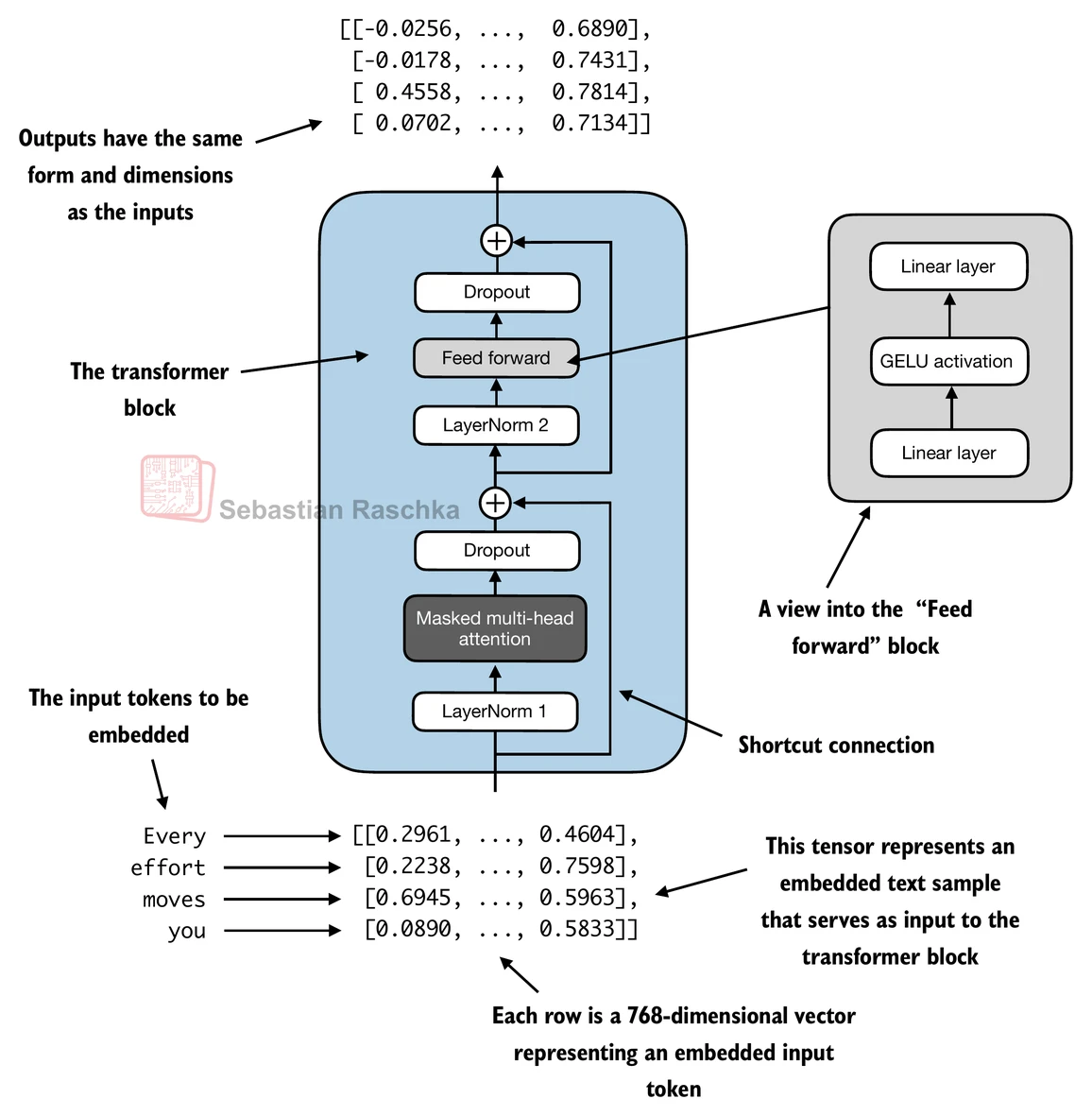
假设我们有2个输入样本，每个有6个token，其中每个token是一个768维的嵌入向量；那么这个transformer块应用自注意力，然后是线性层，产生类似大小的输出
你可以将输出视为我们在前一章中讨论的上下文向量的增强版本

torch.manual_seed(123)

x = torch.rand(2, 4, 768)  # 形状: [batch_size, num_tokens, emb_dim]
block = TransformerBlock(GPT_CONFIG_124M)
output = block(x)

print("Input shape:", x.shape)
print("Output shape:", output.shape)

Input shape: torch.Size([2, 4, 768])
Output shape: torch.Size([2, 4, 768])

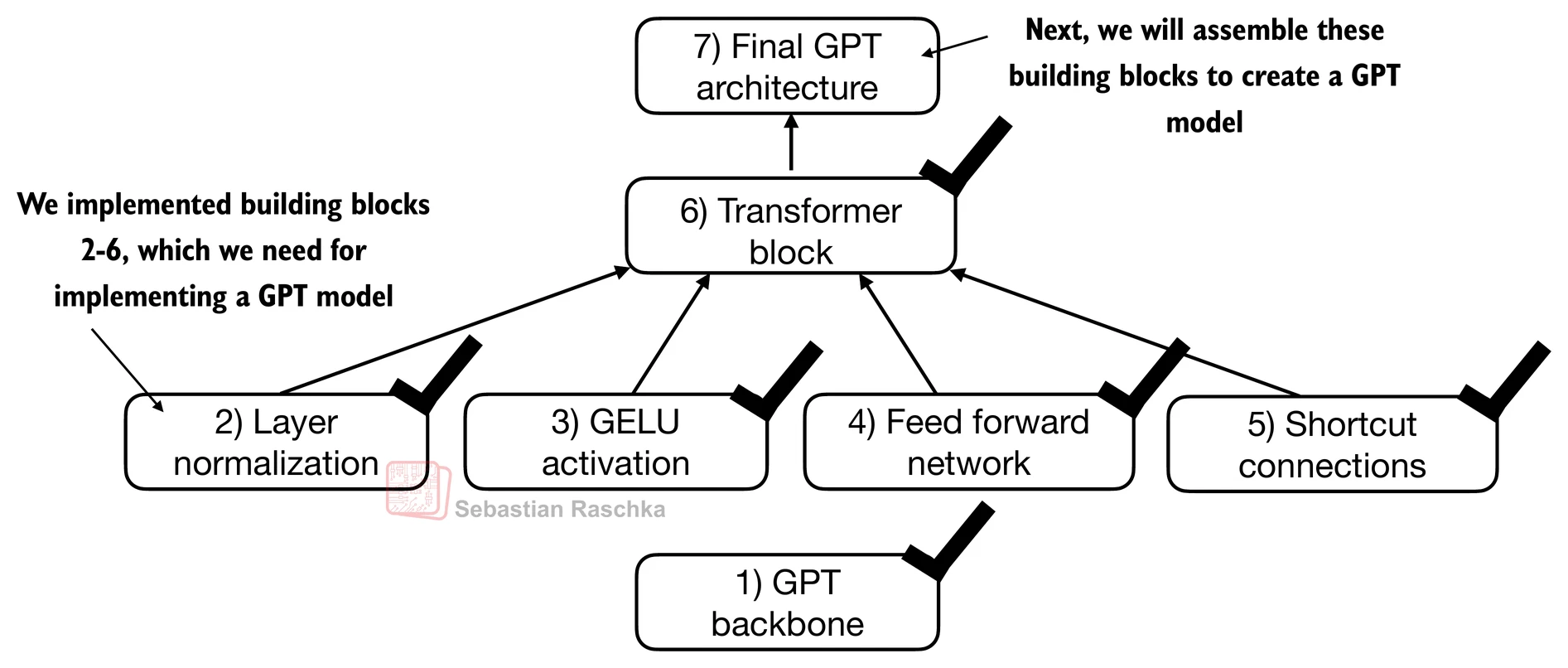
4.6 编写GPT模型代码

我们快到了：现在让我们将transformer块插入到本章开头编写的架构中，这样我们就得到了一个可用的GPT架构
注意transformer块会重复多次；在最小的124M GPT-2模型的情况下，我们重复它12次：

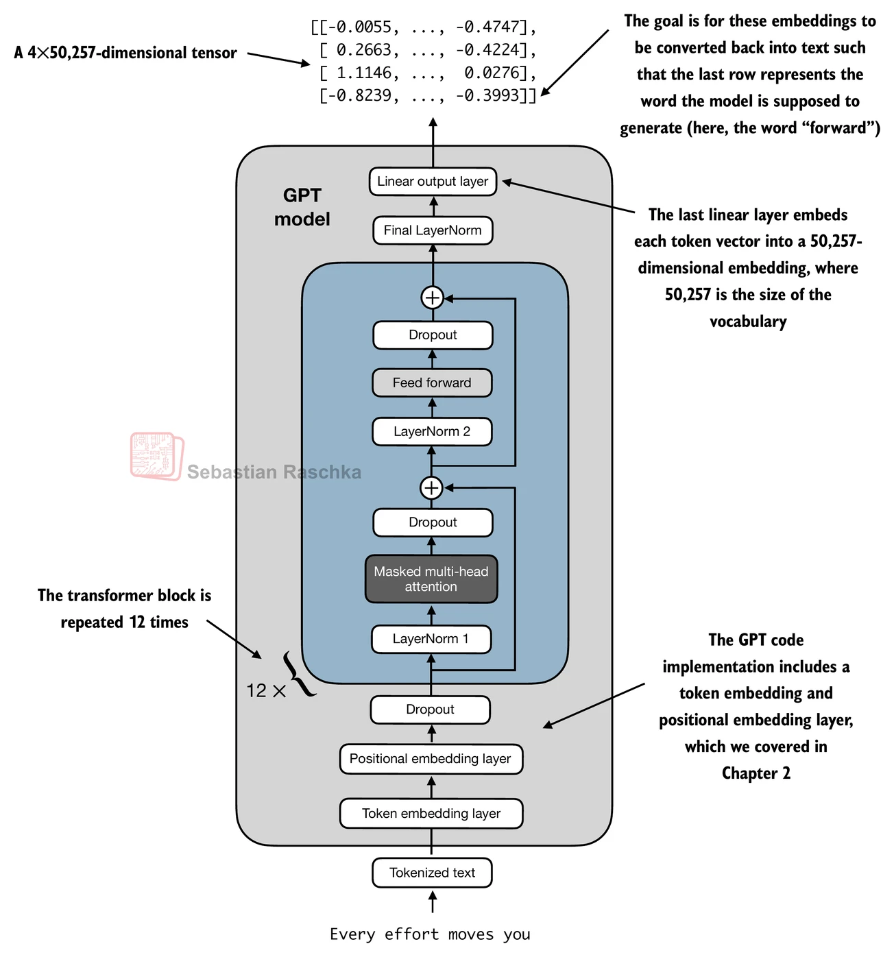
相应的代码实现，其中cfg["n_layers"] = 12：

class GPTModel(nn.Module):
    def __init__(self, cfg):
        super().__init__()
        self.tok_emb = nn.Embedding(cfg["vocab_size"], cfg["emb_dim"])
        self.pos_emb = nn.Embedding(cfg["context_length"], cfg["emb_dim"])
        self.drop_emb = nn.Dropout(cfg["drop_rate"])
        
        self.trf_blocks = nn.Sequential(
            *[TransformerBlock(cfg) for _ in range(cfg["n_layers"])])
        
        self.final_norm = LayerNorm(cfg["emb_dim"])
        self.out_head = nn.Linear(
            cfg["emb_dim"], cfg["vocab_size"], bias=False
        )

    def forward(self, in_idx):
        batch_size, seq_len = in_idx.shape
        tok_embeds = self.tok_emb(in_idx)
        pos_embeds = self.pos_emb(torch.arange(seq_len, device=in_idx.device))
        x = tok_embeds + pos_embeds  # 形状 [batch_size, num_tokens, emb_size]
        x = self.drop_emb(x)
        x = self.trf_blocks(x)
        x = self.final_norm(x)
        logits = self.out_head(x)
        return logits

使用124M参数模型的配置，我们现在可以用随机初始权重实例化这个GPT模型，如下所示：

torch.manual_seed(123)
model = GPTModel(GPT_CONFIG_124M)

out = model(batch)
print("Input batch:\n", batch)
print("\nOutput shape:", out.shape)
print(out)

Input batch:
 tensor([[6109, 3626, 6100,  345],
        [6109, 1110, 6622,  257]])

Output shape: torch.Size([2, 4, 50257])
tensor([[[ 0.1381,  0.0077, -0.1963,  ..., -0.0222, -0.1060,  0.1717],
         [ 0.3865, -0.8408, -0.6564,  ..., -0.5163,  0.2369, -0.3357],
         [ 0.6989, -0.1829, -0.1631,  ...,  0.1472, -0.6504, -0.0056],
         [-0.4290,  0.1669, -0.1258,  ...,  1.1579,  0.5303, -0.5549]],

        [[ 0.1094, -0.2894, -0.1467,  ..., -0.0557,  0.2911, -0.2824],
         [ 0.0882, -0.3552, -0.3527,  ...,  1.2930,  0.0053,  0.1898],
         [ 0.6091,  0.4702, -0.4094,  ...,  0.7688,  0.3787, -0.1974],
         [-0.0612, -0.0737,  0.4751,  ...,  1.2463, -0.3834,  0.0609]]],
       grad_fn=<UnsafeViewBackward0>)

我们将在下一章训练这个模型
但是，关于其大小的一个快速说明：我们之前称它为124M参数模型；我们可以如下双重检查这个数字：

total_params = sum(p.numel() for p in model.parameters())
print(f"参数总数: {total_params:,}")

参数总数: 163,009,536

如我们上面所见，这个模型有163M，而不是124M参数；为什么？
在原始GPT-2论文中，研究人员应用了权重绑定，这意味着他们重用了token嵌入层（tok_emb）作为输出层，这意味着设置self.out_head.weight = self.tok_emb.weight
token嵌入层将50,257维的独热编码输入token投影到768维的嵌入表示
输出层将768维的嵌入投影回50,257维的表示，这样我们就可以将这些转换回单词（下一节将详细介绍）
因此，嵌入层和输出层具有相同数量的权重参数，正如我们可以根据它们权重矩阵的形状看到的那样
但是，关于其大小的一个快速说明：我们之前称它为124M参数模型；我们可以如下双重检查这个数字：

print("Token嵌入层形状:", model.tok_emb.weight.shape)
print("输出层形状:", model.out_head.weight.shape)

Token嵌入层形状: torch.Size([50257, 768])
输出层形状: torch.Size([50257, 768])

在原始GPT-2论文中，研究人员重用了token嵌入矩阵作为输出矩阵
相应地，如果我们减去输出层的参数数量，我们就得到了一个124M参数模型：

total_params_gpt2 =  total_params - sum(p.numel() for p in model.out_head.parameters())
print(f"考虑权重绑定的可训练参数数量: {total_params_gpt2:,}")

考虑权重绑定的可训练参数数量: 124,412,160

在实践中，我发现不使用权重绑定训练模型更容易，这就是为什么我们在这里没有实现它
但是，当我们在第5章加载预训练权重时，我们将重新审视并应用这个权重绑定的想法
最后，我们可以如下计算模型的内存需求，这可以作为一个有用的参考点：

# 计算总字节大小（假设float32，每个参数4字节）
total_size_bytes = total_params * 4

# 转换为兆字节
total_size_mb = total_size_bytes / (1024 * 1024)

print(f"模型总大小: {total_size_mb:.2f} MB")

模型总大小: 621.83 MB

练习：你也可以尝试以下其他配置，这些配置在GPT-2论文中也有引用。
- GPT2-small（我们已经实现的124M配置）：
  - “emb_dim” = 768
  - “n_layers” = 12
  - “n_heads” = 12
- GPT2-medium:
  - “emb_dim” = 1024
  - “n_layers” = 24
  - “n_heads” = 16
- GPT2-large:
  - “emb_dim” = 1280
  - “n_layers” = 36
  - “n_heads” = 20
- GPT2-XL:
  - “emb_dim” = 1600
  - “n_layers” = 48
  - “n_heads” = 25

4.7 生成文本

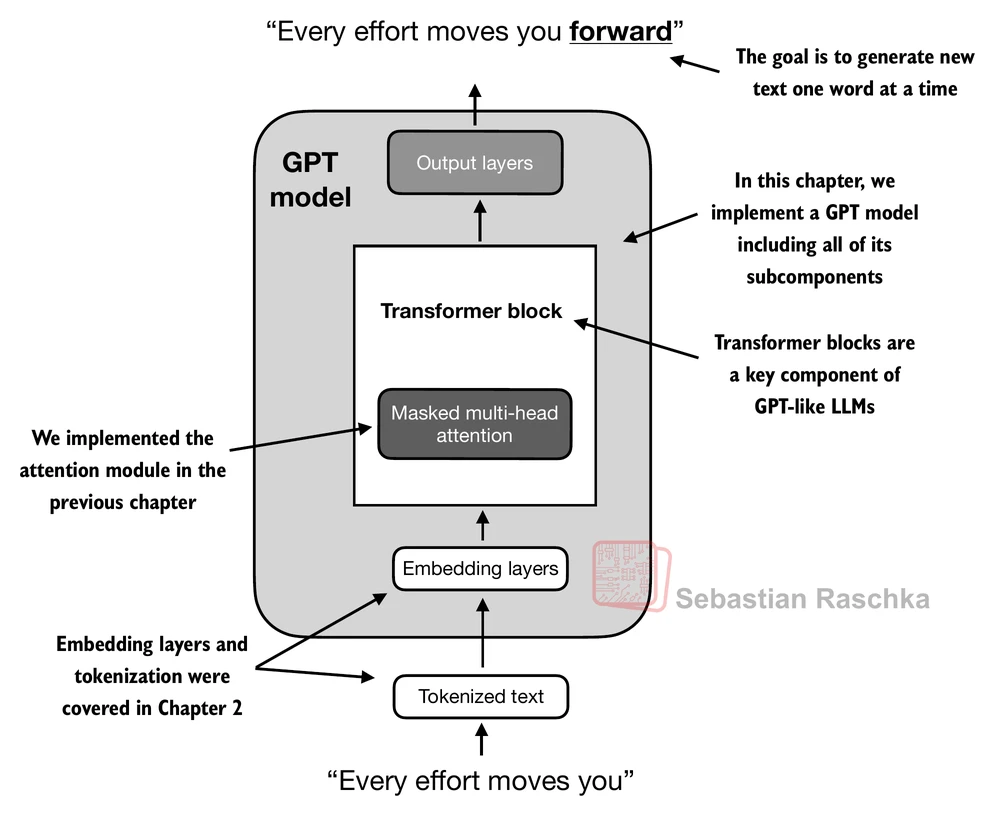
像我们上面实现的GPT模型这样的LLM用于一次生成一个单词

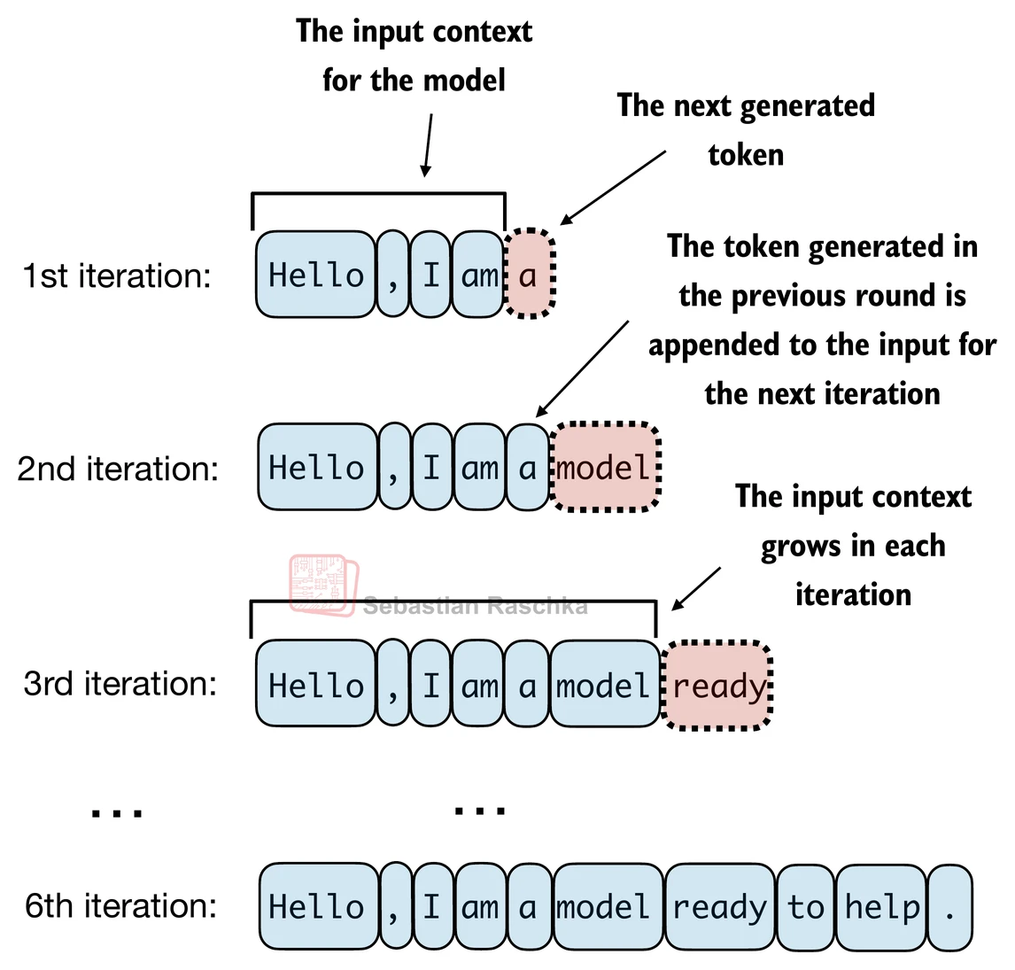
以下generate_text_simple函数实现了贪婪解码，这是一种生成文本的简单快速方法
在贪婪解码中，在每一步，模型选择概率最高的单词（或token）作为其下一个输出（最高的logit对应最高的概率，所以我们技术上甚至不必显式计算softmax函数）
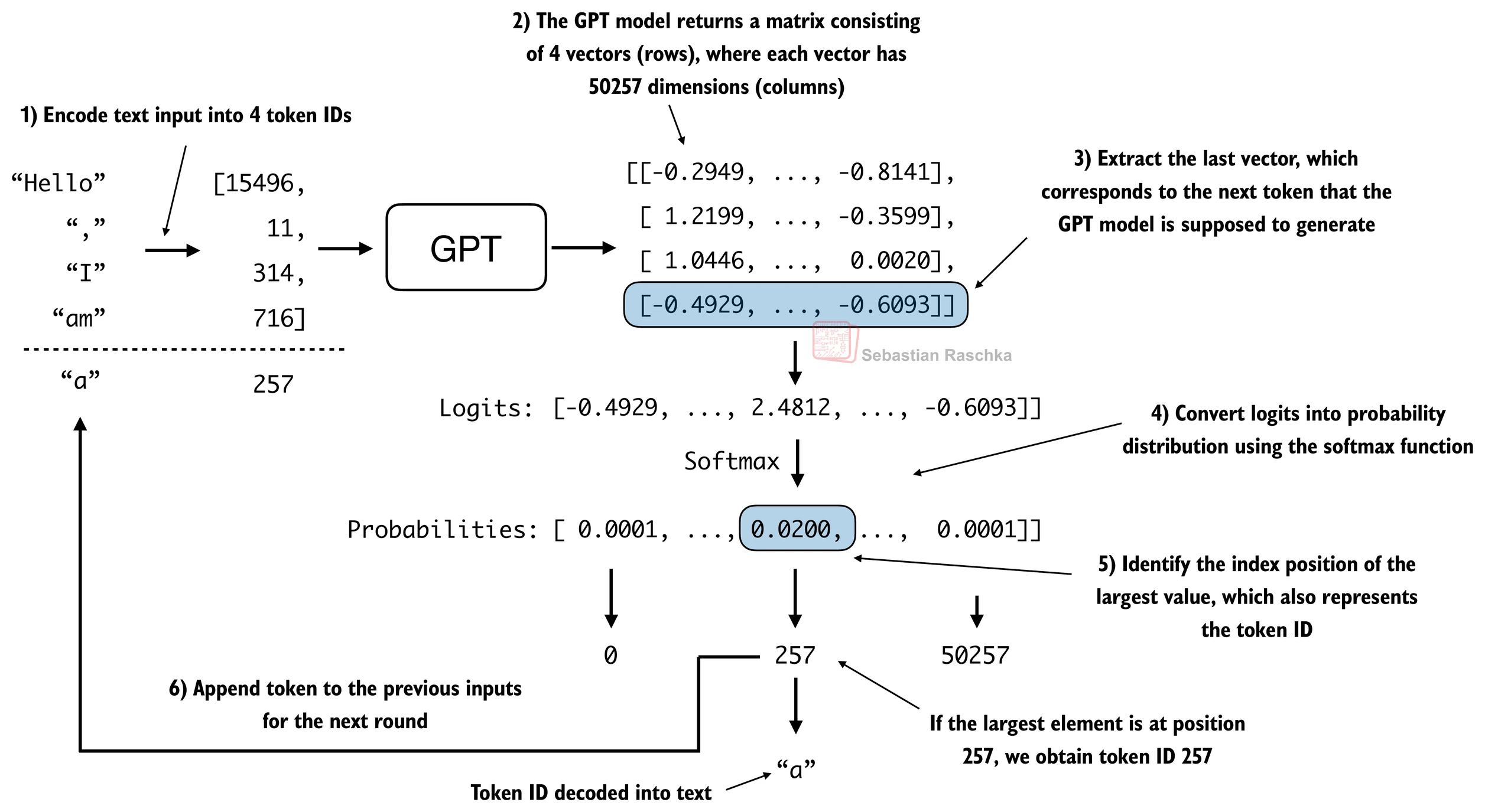
在下一章中，我们将实现一个更高级的generate_text函数
下图描述了GPT模型在给定输入上下文的情况下如何生成下一个单词token

def generate_text_simple(model, idx, max_new_tokens, context_size):
    # idx是当前上下文中索引的(batch, n_tokens)数组
    for _ in range(max_new_tokens):
        
        # 如果当前上下文超过支持的上下文大小，则裁剪它
        # 例如，如果LLM只支持5个token，而上下文大小是10
        # 那么只有最后5个token被用作上下文
        idx_cond = idx[:, -context_size:]
        
        # 获取预测
        with torch.no_grad():
            logits = model(idx_cond)
        
        # 只关注最后一个时间步
        # (batch, n_tokens, vocab_size) 变成 (batch, vocab_size)
        logits = logits[:, -1, :]  

        # 应用softmax获取概率
        probas = torch.softmax(logits, dim=-1)  # (batch, vocab_size)

        # 获取概率值最高的词汇条目的索引
        idx_next = torch.argmax(probas, dim=-1, keepdim=True)  # (batch, 1)

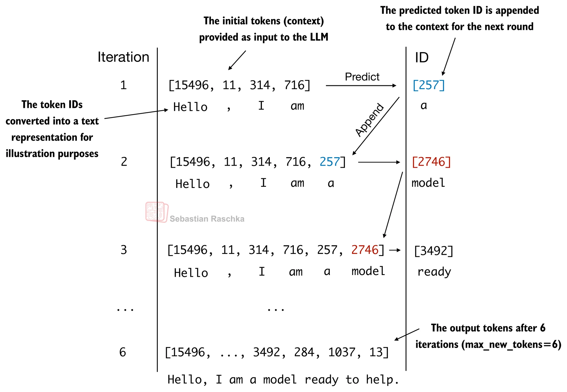
        # 将采样的索引附加到运行序列中
        idx = torch.cat((idx, idx_next), dim=1)  # (batch, n_tokens+1)

    return idx

上面的generate_text_simple实现了一个迭代过程，它一次创建一个token

让我们准备一个输入示例：

start_context = "Hello, I am"

encoded = tokenizer.encode(start_context)
print("encoded:", encoded)

encoded_tensor = torch.tensor(encoded).unsqueeze(0)
print("encoded_tensor.shape:", encoded_tensor.shape)

encoded: [15496, 11, 314, 716]
encoded_tensor.shape: torch.Size([1, 4])

model.eval() # 禁用dropout

out = generate_text_simple(
    model=model,
    idx=encoded_tensor, 
    max_new_tokens=6, 
    context_size=GPT_CONFIG_124M["context_length"]
)

print("Output:", out)
print("Output length:", len(out[0]))

Output: tensor([[15496,    11,   314,   716, 27018, 24086, 47843, 30961, 42348,  7267]])
Output length: 10

移除批次维度并转换回文本：

decoded_text = tokenizer.decode(out.squeeze(0).tolist())
print(decoded_text)

Hello, I am Featureiman Byeswickattribute argue

注意模型是未训练的；因此上面的输出文本是随机的
我们将在下一章训练模型

总结和要点

请参阅./gpt.py脚本，这是一个包含我们在此Jupyter notebook中实现的GPT模型的独立脚本
你可以在./exercise-solutions.ipynb中找到练习解答