Pytorch 注意力机制

Pytorch 注意力机制

0. 环境介绍

环境使用 Kaggle 里免费建立的 Notebook

教程使用李沐老师的 动手学深度学习 网站和 视频讲解

小技巧：当遇到函数看不懂的时候可以按 Shift+Tab 查看函数详解。

1. 注意力

1.1 心理学

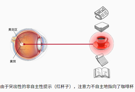
• 动物需要在复杂环境下有效关注值得注意的点
• 心理学框架：人类根据随意线索和不随意线索选择注意点

不随意线索（无意识注意）：

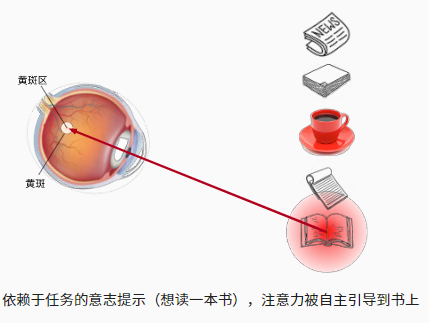
想读书：随意线索（有意识地注意）

1.2 注意力机制

• 卷积、全连接、池化层都只考虑不随意线索（无意识的）
• 注意力机制则显式的考虑随意线索（有意识的）
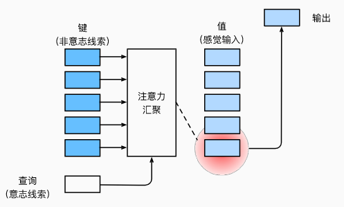
  • 随意线索被称之为查询（Query）
  • 每个输入是一个值（Value）和不随意线索（Key）的对
  • 通过注意力池化（Pooling）来有偏向性的选择某些输入

1.3 非参注意力池化层

非参就是不学习参数。

• 给定数据 $(x_i,y_i),i=1,...,n$
• 平均池化是最简单的方案：
  $$f(x)=\frac{1}{n}\sum _i{y}_i$$
• 更好的方案是 60 年代提出来的 Nadaraya-Watson 核回归
  $$f(x)=\sum _{i=1}^n\frac{K\left(x-x_i\right)}{{\sum }_{j=1}^{n}K\left(x-x_j\right)}{y}_i$$
  $x$ 表示 Query，$x_j,x_i$ 表示 Key，$y_i$ 表示 Value。

1.4 Nadaraya-Watson 核回归

• 如果 使用高斯核：
  $$K(u)=\frac{1}{\sqrt{2\pi }}\exp \left(-\frac{u^2}{2}\right)$$
• 那么：
  $$\begin{array}{rl}f(x)& =\sum _{i=1}^n\frac{\exp \left(-\frac{1}{2}{\left(x-x_i\right)}^2\right)}{{\sum }_{j=1}^n\exp \left(-\frac{1}{2}{\left(x-x_j\right)}^2\right)}{y}_i\\ & =\sum _{i=1}^n\mathrm{softmax}\left(-\frac{1}{2}{\left(x-x_i\right)}^2\right)y_i\end{array}$$

1.5 参数化的注意力机制

• 在 1.4 的基础上引入可学系的权重 $w$：
  $$f(x)=\sum _{i=1}^n\mathrm{softmax}\left(-\frac{1}{2}{\left(\left(x-x_i\right)w\right)}^2\right)y_i$$

• 可以一般化写作 $f(x)={\sum }_i\alpha \left(x,x_i\right)y_i$，这里 $\alpha \left(x,x_i\right)$ 是注意力权重。

注意力机制关键就在于权重如何设计。

2. 代码

2.0 导包

!pip install -U d2l
import torch
from torch import nn
from d2l import torch as d2l

2.1 生成数据集

考虑一个回归问题：给定成对的 “输入-输出” 数据集 { ( x 1 , y 1 ) , . . . , ( x n , y n ) } \{(x_1, y_1), ..., (x_n, y_n)\} {(x1​,y1​),...,(xn​,yn​)}，如何学习 $f$ 来预测任意新的输入 $x$ 的输出 $\hat{y}=f(x)$？

根据下面的非线性函数生成一个人工数据集， 其中加入的噪声项为 $ϵ$：
$$y_i=2\sin (x_i)+x_i^{0.8}+ϵ$$
其中噪声项 $ϵ\sim N(0,0.5^2)$

n_train = 50  # 训练样本数
# 排序后的训练样本
x_train, _ = torch.sort(torch.rand(n_train) * 5)   

def f(x):
    return 2 * torch.sin(x) + x**0.8

y_train = f(x_train) + torch.normal(0.0, 0.5, (n_train,))  # 训练样本的输出

# 测试样本
x_test = torch.arange(0, 5, 0.1)  
y_truth = f(x_test)  # 测试样本的真实输出
n_test = len(x_test)  # 测试样本数
n_test

2.2 定义绘制所有训练样本的函数

def plot_kernel_reg(y_hat):
    d2l.plot(x_test, [y_truth, y_hat], 'x', 'y', legend=['Truth', 'Pred'],
             xlim=[0, 5], ylim=[-1, 5])
    d2l.plt.plot(x_train, y_train, 'o', alpha=0.5);

2.3 平均汇聚（Pooling）

y_hat = torch.repeat_interleave(y_train.mean(), n_test)
plot_kernel_reg(y_hat)

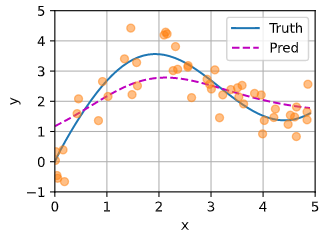
黄色的点表示训练的点，蓝线表示真实值，红色虚线表示最简单的平均线作为预测（不靠谱）。

2.3 非参数注意力汇聚（Pooling）

使用高斯核：

# X_repeat的形状:(n_test,n_train),
# 每一行都包含着相同的测试输入（例如：同样的查询）
X_repeat = x_test.repeat_interleave(n_train).reshape((-1, n_train))
# x_train包含着键。attention_weights的形状：(n_test,n_train),
# 每一行都包含着要在给定的每个查询的值（y_train）之间分配的注意力权重
attention_weights = nn.functional.softmax(-(X_repeat - x_train)**2 / 2, dim=1)
# y_hat的每个元素都是值的加权平均值，其中的权重是注意力权重
y_hat = torch.matmul(attention_weights, y_train)
plot_kernel_reg(y_hat)

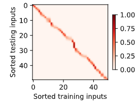
2.4 注意力权重

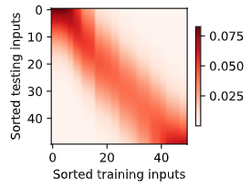
这里测试数据的输入相当于查询（Query），而训练数据的输入相当于键（Key）。 因为两个输入都是经过排序的，因此由观察可知 “查询-键” 对（Q-K）越接近， 注意力汇聚的注意力权重就越高。

d2l.show_heatmaps(attention_weights.unsqueeze(0).unsqueeze(0),
                  xlabel='Sorted training inputs',
                  ylabel='Sorted testing inputs')

2.5 带参数注意力池化（Pooling）

假定两个张量的形状分别是 $(n,a,b)$ 和 $(n,b,c)$，它们的批量矩阵乘法输出的形状为 $(n,a,c)$：

X = torch.ones((2, 1, 4))
Y = torch.ones((2, 4, 6))
# bmm 表示批量矩阵乘法函数
torch.bmm(X, Y).shape

2.5.1 定义模型

class NWKernelRegression(nn.Module):
    def __init__(self, **kwargs):
        super().__init__(**kwargs)
        self.w = nn.Parameter(torch.rand((1,), requires_grad=True))

    def forward(self, queries, keys, values):
        # queries和attention_weights的形状为(查询个数，“键－值”对个数)
        queries = queries.repeat_interleave(keys.shape[1]).reshape((-1, keys.shape[1]))
        self.attention_weights = nn.functional.softmax(
            -((queries - keys) * self.w)**2 / 2, dim=1)
        # values的形状为(查询个数，“键－值”对个数)
        return torch.bmm(self.attention_weights.unsqueeze(1),
                         values.unsqueeze(-1)).reshape(-1)

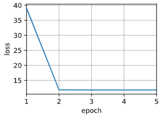
2.5.2 训练

# X_tile的形状:(n_train，n_train)，每一行都包含着相同的训练输入
X_tile = x_train.repeat((n_train, 1))
# Y_tile的形状:(n_train，n_train)，每一行都包含着相同的训练输出
Y_tile = y_train.repeat((n_train, 1))
# keys的形状:('n_train'，'n_train'-1)
keys = X_tile[(1 - torch.eye(n_train)).type(torch.bool)].reshape((n_train, -1))
# values的形状:('n_train'，'n_train'-1)
values = Y_tile[(1 - torch.eye(n_train)).type(torch.bool)].reshape((n_train, -1))

net = NWKernelRegression()
loss = nn.MSELoss(reduction='none')
trainer = torch.optim.SGD(net.parameters(), lr=0.5)
animator = d2l.Animator(xlabel='epoch', ylabel='loss', xlim=[1, 5])

for epoch in range(5):
    trainer.zero_grad()
    l = loss(net(x_train, keys, values), y_train)
    l.sum().backward()
    trainer.step()
    print(f'epoch {epoch + 1}, loss {float(l.sum()):.6f}')
    animator.add(epoch + 1, float(l.sum()))

预测结果绘制的线不如之前非参数模型的平滑：

# keys的形状:(n_test，n_train)，每一行包含着相同的训练输入（例如，相同的键）
keys = x_train.repeat((n_test, 1))
# value的形状:(n_test，n_train)
values = y_train.repeat((n_test, 1))
y_hat = net(x_test, keys, values).unsqueeze(1).detach()
plot_kernel_reg(y_hat)

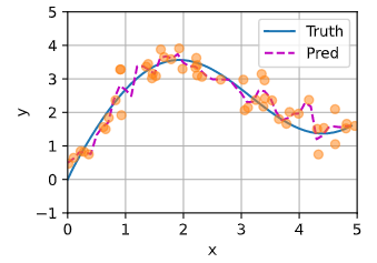
与非参数的注意力汇聚模型相比， 带参数的模型加入可学习的参数后， 曲线在注意力权重较大的区域变得更不平滑：

d2l.show_heatmaps(net.attention_weights.unsqueeze(0).unsqueeze(0),
                  xlabel='Sorted training inputs',
                  ylabel='Sorted testing inputs')