


 本文深入探讨Pandas和NumPy在数据筛选、更改、整合、导入导出及可视化方面的应用,涵盖多种数据操作方法,如loc、iloc、fillna、merge等,适合初学者及有经验的数据分析师。
python数据处理之numpy和pandas(下)
2.三种数据筛选方式
pandas筛选数据是比较好用的,至少比Excel要好一些,再加上可视化的数据模块,简直是大数据中的一把处理利器。值得一提的是曾经pandas中又一个很好用的.ix数据筛选方法,但是会在实际使用的过程中出现歧义,就被新版本的弃用了,所以现在是永不了.ix去筛选数据的。下面我们就开始介绍着四种数据筛选方式,都在代码里面贴出:
- import numpy as np
- import pandas as pd
-
- dates = pd.date_range('20171010', periods=6)
- df = pd.DataFrame(np.arange(24).reshape((6,4)), index = dates, columns=['A','B','C','D'])
- print(df)
- #普通的筛选方式
- print("普通的筛选方式")
- print(df['A'],df.A)
- print(df[0:3],df['20171010':'20171012'])
- #基于loc的筛选
- print("基于loc的筛选")
- print(df.loc['20171010'])
- print(df.loc[:,['A','C']])
- print(df.loc['20171010',['A','C']])
- #基于iloc的筛选
- print("基于iloc的筛选")
- print(df.iloc[3,1])
- print(df.iloc[3:5,1:3])
- print(df.iloc[[1,3,5,],1:3])
- #基于条件筛选
- print("基于条件筛选")
- print(df[df.B>8])
- A B C D
- 2017-10-10 0 1 2 3
- 2017-10-11 4 5 6 7
- 2017-10-12 8 9 10 11
- 2017-10-13 12 13 14 15
- 2017-10-14 16 17 18 19
- 2017-10-15 20 21 22 23
- 普通的筛选方式
- 2017-10-10 0
- 2017-10-11 4
- 2017-10-12 8
- 2017-10-13 12
- 2017-10-14 16
- 2017-10-15 20
- Freq: D, Name: A, dtype: int32 2017-10-10 0
- 2017-10-11 4
- 2017-10-12 8
- 2017-10-13 12
- 2017-10-14 16
- 2017-10-15 20
- Freq: D, Name: A, dtype: int32
- A B C D
- 2017-10-10 0 1 2 3
- 2017-10-11 4 5 6 7
- 2017-10-12 8 9 10 11 A B C D
- 2017-10-10 0 1 2 3
- 2017-10-11 4 5 6 7
- 2017-10-12 8 9 10 11
- 基于loc的筛选
- A 0
- B 1
- C 2
- D 3
- Name: 2017-10-10 00:00:00, dtype: int32
- A C
- 2017-10-10 0 2
- 2017-10-11 4 6
- 2017-10-12 8 10
- 2017-10-13 12 14
- 2017-10-14 16 18
- 2017-10-15 20 22
- A 0
- C 2
- Name: 2017-10-10 00:00:00, dtype: int32
- 基于iloc的筛选
- 13
- B C
- 2017-10-13 13 14
- 2017-10-14 17 18
- B C
- 2017-10-11 5 6
- 2017-10-13 13 14
- 2017-10-15 21 22
- 基于条件筛选
- A B C D
- 2017-10-12 8 9 10 11
- 2017-10-13 12 13 14 15
- 2017-10-14 16 17 18 19
- 2017-10-15 20 21 22 23
3.数据更改
对于已知的pandas数组,如果想要更改它其中的数据,方法是有的而且还不少,现在我们就开始先介绍一下吧:
- import numpy as np
- import pandas as pd
-
- dates = pd.date_range('20171010',periods=6)
- df = pd.DataFrame(np.arange(24).reshape((6,4)), index = dates, columns=['A','B','C','D'])
- print(df)
- df.iloc[2,2] = 1111
- print(df)
- df.loc['20171013','C'] = 2222
- print(df)
- df.B[df.A>4] = 0
- print(df)
- df['F'] = 0
- print(df)
- df['G'] = pd.Series([1,2,3,4,5,6],index=pd.date_range('20171010',periods=6))
- print(df)
如上代码所示,先建立一个数据矩阵,列索引用日期,行索引用大写字母。如果想改变数据中的某个值即单值改变,那么比较恰到的方法当然是上面所要提到的loc和iloc,loc索引是需要写出来索引的名字而iloc只需要填写坐标,我个人还是倾向于填写坐标的方式来进行改写数据,改变某个值就直接复制好了,十分方便的。如果你在图像处理的过程中想设定阈值对里面的数据进行判别,就需要条件设置了,这种方法在上文中有所提到,即判断A列数值是否大于4,找出大于4的若干行,在这几行中B列的元素全部置零。如果批量处理某些整行或者整列的话就则需要像上面代码里面所描述的那,只需要赋值一个数就代表整列,若是这一列都是不同的数值就需要用iloc了。还可以通过Series序列去添加数据,依然是可以的。下面将结果显示出来:
- A B C D
- 2017-10-10 0 1 2 3
- 2017-10-11 4 5 6 7
- 2017-10-12 8 9 10 11
- 2017-10-13 12 13 14 15
- 2017-10-14 16 17 18 19
- 2017-10-15 20 21 22 23
- A B C D
- 2017-10-10 0 1 2 3
- 2017-10-11 4 5 6 7
- 2017-10-12 8 9 1111 11
- 2017-10-13 12 13 14 15
- 2017-10-14 16 17 18 19
- 2017-10-15 20 21 22 23
- A B C D
- 2017-10-10 0 1 2 3
- 2017-10-11 4 5 6 7
- 2017-10-12 8 9 1111 11
- 2017-10-13 12 13 2222 15
- 2017-10-14 16 17 18 19
- 2017-10-15 20 21 22 23
- A B C D
- 2017-10-10 0 1 2 3
- 2017-10-11 4 5 6 7
- 2017-10-12 8 0 1111 11
- 2017-10-13 12 0 2222 15
- 2017-10-14 16 0 18 19
- 2017-10-15 20 0 22 23
- A B C D F
- 2017-10-10 0 1 2 3 0
- 2017-10-11 4 5 6 7 0
- 2017-10-12 8 0 1111 11 0
- 2017-10-13 12 0 2222 15 0
- 2017-10-14 16 0 18 19 0
- 2017-10-15 20 0 22 23 0
- A B C D F G
- 2017-10-10 0 1 2 3 0 1
- 2017-10-11 4 5 6 7 0 2
- 2017-10-12 8 0 1111 11 0 3
- 2017-10-13 12 0 2222 15 0 4
- 2017-10-14 16 0 18 19 0 5
- 2017-10-15 20 0 22 23 0 6
4.数据整合和处理
在处理一些数据的过程中,可能会出现一些数据块是空的或者为np.NaN的类型,如何删除或者是填补这些数据呢,下面需要提及的就是几个相对好用的函数:
- import numpy as np
- import pandas as pd
-
- dates = pd.date_range('20171010',periods=6)
- df = pd.DataFrame(np.arange(24).reshape((6,4)),index=dates,columns=['A','B','C','D'])
- df.iloc[0,1]=np.nan
- df.iloc[1,2]=np.nan
- print(df)
- print(df.dropna(axis=0,how='any'))
- print(df.fillna(value=1111))
- print(df.isnull())
- print(np.any(df.isnull())==True)
- A B C D
- 2017-10-10 0 NaN 2.0 3
- 2017-10-11 4 5.0 NaN 7
- 2017-10-12 8 9.0 10.0 11
- 2017-10-13 12 13.0 14.0 15
- 2017-10-14 16 17.0 18.0 19
- 2017-10-15 20 21.0 22.0 23
- A B C D
- 2017-10-12 8 9.0 10.0 11
- 2017-10-13 12 13.0 14.0 15
- 2017-10-14 16 17.0 18.0 19
- 2017-10-15 20 21.0 22.0 23
- A B C D
- 2017-10-10 0 1111.0 2.0 3
- 2017-10-11 4 5.0 1111.0 7
- 2017-10-12 8 9.0 10.0 11
- 2017-10-13 12 13.0 14.0 15
- 2017-10-14 16 17.0 18.0 19
- 2017-10-15 20 21.0 22.0 23
- A B C D
- 2017-10-10 False True False False
- 2017-10-11 False False True False
- 2017-10-12 False False False False
- 2017-10-13 False False False False
- 2017-10-14 False False False False
- 2017-10-15 False False False False
- True
5.数据的导入和导出
如果用pandas从本地导入一个文件(其支持的数据文件格式有很多种,在机器学习领域我们用的最多的还是CSV文件,在进行神经网络训练的时候,我们进行数据存储就是此种格式),要想读取一个文件则使用pd.read_csv(‘文件名’),想要写入一个文件则使用to_文件格式(‘文件名’),在这里需要着重提的是文件路径一定要正确。下面将代码和运行结果打印出来:
- import pandas as pd
- data = pd.read_csv('student.csv')
- print(data)
- data.to_pickle('student.pickle')
- Student ID name age gender
- 0 1100 Kelly 22 Female
- 1 1101 Clo 21 Female
- 2 1102 Tilly 22 Female
- 3 1103 Tony 24 Male
- 4 1104 David 20 Male
- 5 1105 Catty 22 Female
- 6 1106 M 3 Female
- 7 1107 N 43 Male
- 8 1108 A 13 Male
- 9 1109 S 12 Male
- 10 1110 David 33 Male
- 11 1111 Dw 3 Female
- 12 1112 Q 23 Male
- 13 1113 W 21 Female
6.pandas数据合并
数据合并是一个非常重要的数据操作手段,下面会介绍两种形式的数据合并,第一种是基于concat的:
- import numpy as np
- import pandas as pd
- #concatenating
- df1 = pd.DataFrame(np.ones((3,4))*0, columns=['A','B','C','D'])
- df2 = pd.DataFrame(np.ones((3,4))*1, columns=['A','B','C','D'])
- df3 = pd.DataFrame(np.ones((3,4))*2, columns=['A','B','C','D'])
- print(df1)
- print(df2)
- print(df3)
- res = pd.concat([df1,df2,df3], axis=0, ignore_index=True)
- print(res)
- #join['inner','outer']
- df1 = pd.DataFrame(np.ones((3,4))*0, columns=['A','B','C','D'], index=[1,2,3])
- df2 = pd.DataFrame(np.ones((3,4))*1, columns=['B','C','D','E'], index=[2,3,4])
- print(df1)
- print(df2)
- res = pd.concat([df1,df2],join='inner', ignore_index=True)
- print(res)
- df1 = pd.DataFrame(np.ones((3,4))*0, columns=['A','B','C','D'], index=[1,2,3])
- df2 = pd.DataFrame(np.ones((3,4))*1, columns=['B','C','D','E'], index=[2,3,4])
- print(df1)
- print(df2)
- res = pd.concat([df1,df2],axis=1,join_axes=[df1.index])
- print(res)
- df1 = pd.DataFrame(np.ones((3,4))*0, columns=['A','B','C','D'])
- df2 = pd.DataFrame(np.ones((3,4))*1, columns=['A','B','C','D'])
- df3 = pd.DataFrame(np.ones((3,4))*1, columns=['A','B','C','D'])
- print(df1)
- res = df1.append([df2,df3], ignore_index=True)
- print(res)
- df1 = pd.DataFrame(np.ones((3,4))*0, columns=['A','B','C','D'])
- s1=pd.Series([1,2,3,4],index=['A','B','C','D'])
- res = df1.append(s1,ignore_index=True)
- print(res)
- A B C D
- 0 0.0 0.0 0.0 0.0
- 1 0.0 0.0 0.0 0.0
- 2 0.0 0.0 0.0 0.0
- A B C D
- 0 1.0 1.0 1.0 1.0
- 1 1.0 1.0 1.0 1.0
- 2 1.0 1.0 1.0 1.0
- A B C D
- 0 2.0 2.0 2.0 2.0
- 1 2.0 2.0 2.0 2.0
- 2 2.0 2.0 2.0 2.0
- A B C D
- 0 0.0 0.0 0.0 0.0
- 1 0.0 0.0 0.0 0.0
- 2 0.0 0.0 0.0 0.0
- 3 1.0 1.0 1.0 1.0
- 4 1.0 1.0 1.0 1.0
- 5 1.0 1.0 1.0 1.0
- 6 2.0 2.0 2.0 2.0
- 7 2.0 2.0 2.0 2.0
- 8 2.0 2.0 2.0 2.0
- A B C D
- 1 0.0 0.0 0.0 0.0
- 2 0.0 0.0 0.0 0.0
- 3 0.0 0.0 0.0 0.0
- B C D E
- 2 1.0 1.0 1.0 1.0
- 3 1.0 1.0 1.0 1.0
- 4 1.0 1.0 1.0 1.0
- B C D
- 0 0.0 0.0 0.0
- 1 0.0 0.0 0.0
- 2 0.0 0.0 0.0
- 3 1.0 1.0 1.0
- 4 1.0 1.0 1.0
- 5 1.0 1.0 1.0
- A B C D
- 1 0.0 0.0 0.0 0.0
- 2 0.0 0.0 0.0 0.0
- 3 0.0 0.0 0.0 0.0
- B C D E
- 2 1.0 1.0 1.0 1.0
- 3 1.0 1.0 1.0 1.0
- 4 1.0 1.0 1.0 1.0
- A B C D B C D E
- 1 0.0 0.0 0.0 0.0 NaN NaN NaN NaN
- 2 0.0 0.0 0.0 0.0 1.0 1.0 1.0 1.0
- 3 0.0 0.0 0.0 0.0 1.0 1.0 1.0 1.0
- A B C D
- 0 0.0 0.0 0.0 0.0
- 1 0.0 0.0 0.0 0.0
- 2 0.0 0.0 0.0 0.0
- A B C D
- 0 0.0 0.0 0.0 0.0
- 1 0.0 0.0 0.0 0.0
- 2 0.0 0.0 0.0 0.0
- 3 1.0 1.0 1.0 1.0
- 4 1.0 1.0 1.0 1.0
- 5 1.0 1.0 1.0 1.0
- 6 1.0 1.0 1.0 1.0
- 7 1.0 1.0 1.0 1.0
- 8 1.0 1.0 1.0 1.0
- A B C D
- 0 0.0 0.0 0.0 0.0
- 1 0.0 0.0 0.0 0.0
- 2 0.0 0.0 0.0 0.0
- 3 1.0 2.0 3.0 4.0
- import pandas as pd
-
- left = pd.DataFrame({'key1':['K0','K0','K1','K2'],
- 'key2':['K0','K1','K0','K1'],
- 'A':['A0','A1','A2','A3'],
- 'B':['B0','B1','B2','B3']})
- right = pd.DataFrame({'key1':['K0','K1','K1','K2'],
- 'key2':['K0','K0','K0','K0'],
- 'C':['C0','C1','C2','C3'],
- 'D':['D0','D1','D2','D3']})
- print(left)
- print(right)
- res = pd.merge(left, right, on=['key1','key2'],how='inner')
- print(res)
- res = pd.merge(left, right, on=['key1','key2'],how='outer')
- print(res)
- res = pd.merge(left, right, on=['key1','key2'],how='left')
- print(res)
- res = pd.merge(left, right, on=['key1','key2'],how='right')
- print(res)
- A B key1 key2
- 0 A0 B0 K0 K0
- 1 A1 B1 K0 K1
- 2 A2 B2 K1 K0
- 3 A3 B3 K2 K1
- C D key1 key2
- 0 C0 D0 K0 K0
- 1 C1 D1 K1 K0
- 2 C2 D2 K1 K0
- 3 C3 D3 K2 K0
- A B key1 key2 C D
- 0 A0 B0 K0 K0 C0 D0
- 1 A2 B2 K1 K0 C1 D1
- 2 A2 B2 K1 K0 C2 D2
- A B key1 key2 C D
- 0 A0 B0 K0 K0 C0 D0
- 1 A1 B1 K0 K1 NaN NaN
- 2 A2 B2 K1 K0 C1 D1
- 3 A2 B2 K1 K0 C2 D2
- 4 A3 B3 K2 K1 NaN NaN
- 5 NaN NaN K2 K0 C3 D3
- A B key1 key2 C D
- 0 A0 B0 K0 K0 C0 D0
- 1 A1 B1 K0 K1 NaN NaN
- 2 A2 B2 K1 K0 C1 D1
- 3 A2 B2 K1 K0 C2 D2
- 4 A3 B3 K2 K1 NaN NaN
- A B key1 key2 C D
- 0 A0 B0 K0 K0 C0 D0
- 1 A2 B2 K1 K0 C1 D1
- 2 A2 B2 K1 K0 C2 D2
- 3 NaN NaN K2 K0 C3 D3
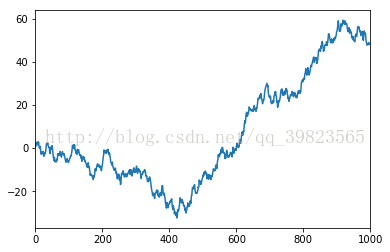
7.数据可视化
数据可视化也是python学习中比较便利的一环,通过matplotlib库可以很轻松的实现饼形图柱状图等深线等高线等数据显示,下面我们来先简单的进行plot的出图:- import pandas as pd
- import numpy as np
- import matplotlib.pyplot as plt
- data = pd.Series(np.random.randn(1000),index=np.arange(1000))
- data = data.cumsum()
- data.plot()
- plt.show()
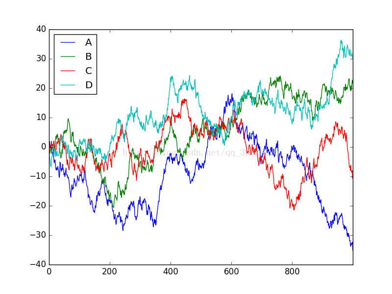
Series只能生成的是一个索引下的可视化,若想生成多条就需要使用DataFrame了,用同样的方法累加就会出现四条不同的数据线:
- import pandas as pd
- import numpy as np
- import matplotlib.pyplot as plt
- data = pd.DataFrame(np.random.randn(1000,4),
- index = np.arange(1000),
- columns=list("ABCD"))
- data=data.cumsum()
- data.plot()
- plt.show()
如果想显示一些散点而不是连接的线,则需要使用scatter函数,通过变量赋值还可以设置散点的颜色参数,标号等,下面就是具体操作:
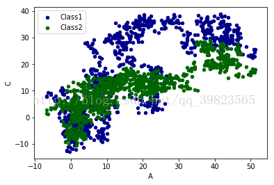
- import pandas as pd
- import numpy as np
- import matplotlib.pyplot as plt
- data = pd.DataFrame(np.random.randn(1000,4),
- index = np.arange(1000),
- columns=list("ABCD"))
- data=data.cumsum()
- ax = data.plot.scatter(x='A',y='B',color='DarkBlue',label='Class1')
- data.plot.scatter(x='A',y='C',color='DarkGreen',label='Class2',ax=ax)
- plt.show()
后记
好了终于咬牙坚持写完了,自己等于又复习了一遍,以上三篇就是numpy和pandas的使用了,这只是一些基本的东西,只有深入到工程之中做一些实际的东西才会大有长进,本来想着将matplotlib也写一下呢,现在看看不必要了,因为在机器学习中这个包用的并不多,只会在计算机视觉领域常见一些吧!当然这是我的猜测和妄语,还请看见的人不要介怀。哎,文章也没人看,不过也好,没人看权当是自己在做笔记,以后真的有问题自己再回来看一下想必也很不错,为了能进烽火或者其他的公司,努力继续前进。加油~~~


 被折叠的 条评论
为什么被折叠?
被折叠的 条评论
为什么被折叠?
 到【灌水乐园】发言


