


 本文介绍线性回归的基本原理及其在房价预测中的应用,详细解析了假设、学习及决策三个阶段,并对比了批量梯度下降与随机梯度下降两种优化算法。
回归
这个概念源于英国生物学家对人类身高的研究。自然界有一种约束力,使人类身高在一定时期是相对稳定的。如果父 母身高矮了(高了),其子女比他们更高(矮),它让身高有一种回归到中心的作用。
linear regression
一个机器学习模型可以划分为三部分。
hypothesis 假设
在这个阶段建立对模型的假设(通常包含未知参数)
learning 学习
构建学习准则(通过优化算法学习得到未知参数)
decision 决策
评判模型的性能
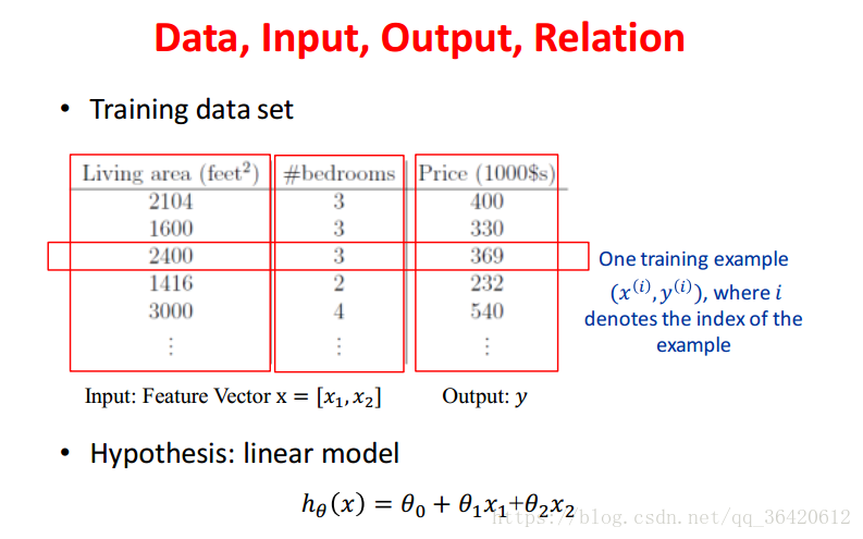
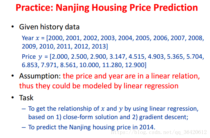
对于图中的房价预测问题,我们建立模型如图。
学习准则是平方误差最小化。
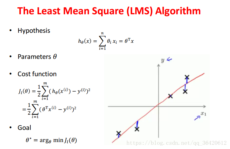
从图中可以看出,平方误差最小化有一个合理的几何解释。它最小化所有样本点到分类面(线)的距离,以期获得最优分类面(线)。
正规方程组法
求解这个问题我们可以直接使用矩阵运算求得结果。
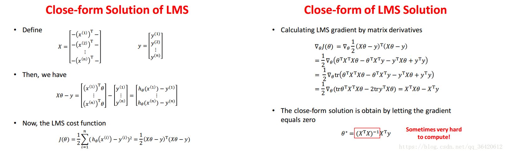
但是,这里涉及到矩阵的逆,难以计算,有时甚至无法计算。
梯度下降法
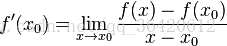
梯度的定义为:
所以,沿着梯度的方向,函数值增大。沿着负梯度方向,函数值降低。梯度下降法是一个迭代算法,不停沿着负梯度方向前进,直到函数值降低到最优解(或局部最优解)或达到停止条件。

这里有个小练习:
import numpy as np
import matplotlib.pyplot as plt
#特征
x = [ i for i in range(14)]
#标签
y = [2.0,2.5,2.9,3.147,4.515,4.903,5.365,5.704,6.853,7.971,8.561,10.0,11.28,12.9]
def loss(w,b):
    #计算损失
    error = 0
    for i in range(len(x)):
        error+=1/2*(w*x[i]+b-y[i])**2
    return error
def batch_gradient_descent(maxCycles,alpha,eps):
    #批量梯度 batch_gradient_descent
    w=0
    b=0
    iter = 0
    error=[]
    for i in range(maxCycles):
        #计算整个数据集的梯度
        sigma1=0
        sigma2=0
        xx= np.linspace(0,14,15)
        ax = fig.add_subplot(2,2,3)
        ax.scatter(x,y,s=30,color='black')
        for i in range(len(x)):
            sigma1 = sigma1 + (w*x[i]+b-y[i])*x[i]
            sigma2= sigma2 + (w*x[i]+b - y[i])
        w = w - sigma1*alpha/len(x)
        b = b - sigma2*alpha/len(x)
        yy=w*xx+b
        plt.plot(xx,yy,color='red',linestyle=':',linewidth=0.5)#画出拟合直线
        plt.xlabel('year')
        plt.ylabel('price')
        plt.title('batch gradient descent')
        iter = iter +1
        error.append(loss(w,b))
        xx = [i for i in range(len(error))]
        ax = fig.add_subplot(2,2,4)
        plt.plot(xx,error,c='red')
        plt.xlabel('iterations')
        plt.ylabel('error')
        plt.title('batch error')
        if loss(w,b)<eps:
            break
    print('批量迭代=',iter,'w=',w,'b=',b,'14年房价=',w*14+b)
    return w,b
def stochastic_gradient_descent(maxCycles,alpha,eps):
    #随机梯度 stochastic_gradient_descent
    iter =0
    w = 0
    b = 0
    flag = 0
    xx= np.linspace(0,14,15)
    ax = fig.add_subplot(2,2,1)
    ax.scatter(x,y,s=30,color='black')
    error=[]
    while True:
        for i in range(len(x)):#循环取数据集中的一个样本计算梯度
            h = w*x[i]+b
            w = w - alpha * (h-y[i]) * x[i]
            b = b - alpha * (h - y[i])
            yy=w*xx+b
            plt.plot(xx,yy,color='blue',linestyle=':',linewidth=0.2)#画出拟合直线
            iter = iter+1
            error.append(loss(w,b))
            if loss(w,b)<eps or iter>=maxCycles:
                flag =1
                break
        if flag:
            break
    plt.xlabel('year')
    plt.ylabel('price')
    plt.title('stochastic gradient descent')
    ax = fig.add_subplot(2,2,2)#画出损失
    xx = [i for i in range(len(error))]
    plt.plot(xx,error)
    plt.xlabel('iterations')
    plt.ylabel('error')
    plt.title('stochastic error')
    print('随机迭代=',iter,'w=',w,'b=',b,'14年房价=',w*14+b)
    return w,b
#初始化参数
maxCycles=200
alpha=0.006
eps = 0.1
#画出数据集
fig = plt.figure()
w1,b1=stochastic_gradient_descent(maxCycles,alpha,eps)
w2,b2=batch_gradient_descent(maxCycles,alpha,eps)
plt.show()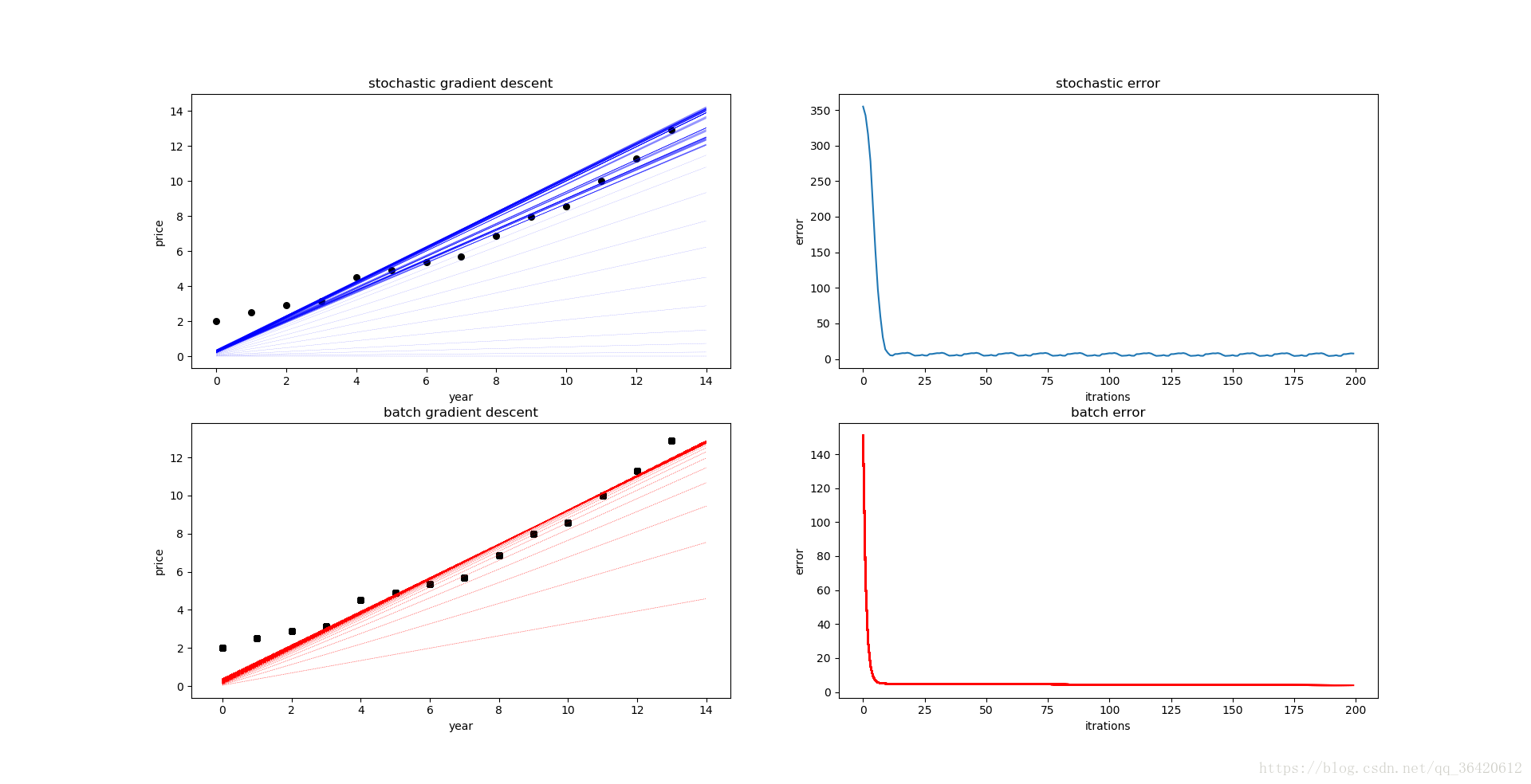


 1万+
1万+

 被折叠的 条评论
为什么被折叠?
被折叠的 条评论
为什么被折叠?
 到【灌水乐园】发言


